MMRR
MMRR_vignette.RmdMultiple matrix regression with randomization (MMRR)
# Install required packages
mmrr_packages()If using MMRR, please cite the following: Wang I.J. (2013) Examining the full effects of landscape heterogeneity on spatial genetic variation: a multiple matrix regression approach for quantifying geographic and ecological isolation. Evolution 67(1):3403-3411. DOI:10.1111/evo.12134
Multiple matrix regression with randomization (Wang 2013) examines how heterogeneity in the landscape (both geographic and environmental) affects spatial genetic variation, allowing a user to determine the relative contributions of isolation by distance (i.e., an association between genetic and geographic distances) and isolation by environment (i.e., an association between genetic and environmental distances). MMRR can provide information concerning how dependent variables (in our case, genetic data) change with respect to multiple independent variables (environmental and geographic distances).
The randomization aspect of MMRR is that significance testing is performed through random permutations of the rows and columns of the dependent matrix (the genetic distances), which is necessary because of the non-independence of values in pairwise distance matrices. Once significance testing is completed, MMRR provides individual regression coefficients and p-values for each dependent variable and a “coefficient ratio,” which is the ratio between regression coefficients, which thus provides an idea of the relative contributions of IBD and IBE in explaining variation in the genetic distances in your data.
There are a few assumptions built into this function that users should be aware of: (1) the coordinates and genetic distance files MUST have the same ordering of individuals; there isn’t a check for this, and (2) this function assumes that each individual has its own sampling coordinates (even if population-based sampling was performed).
Read in and process genetic data
Let’s load the example dataset and extract environmental variables based on our sampling coordinates. To perform MMRR, we need a genetic distance matrix; please refer to the genetic distances vignette for information on how to generate this in algatr using a vcf file.
load_algatr_example()
#>
#> ---------------- example dataset ----------------
#>
#> Objects loaded:
#> *liz_vcf* vcfR object (1000 loci x 53 samples)
#> *liz_gendist* genetic distance matrix (Plink Distance)
#> *liz_coords* dataframe with x and y coordinates
#> *CA_env* RasterStack with example environmental layers
#>
#> -------------------------------------------------
#>
#>
Y <- as.matrix(liz_gendist)
Process environmental data
Let’s calculate environmental distances with our extracted
environmental values using the env_dist() function, and add
on geographic distances to this matrix using the geo_dist()
function. For more information on how these two functions work, please
refer to algatr’s environmental data processing vignette.
Run MMRR
We can run MMRR using the mmrr_run() function. We can
either run the full model (with no variable selection) by setting
model = "full", or by running a variable selection
procedure using backwards elimination by setting
model = "best" within this function. The arguments to
mmrr_run() are as follows:
Y: matrix of genetic distancesX: matrix of environmental distances (including geographic distances) at each sampling coordinatenperm: number of permutations to performstdz: whether matrices are standardized
MMRR with all variables
First, let’s run the full MMRR model with all variables included (i.e., no variable selection).
The results from running the “full” MMRR model contains four elements:
coeff_df: a dataframe with statistics relating to each variable’s distance related to genetic distance, including coefficient values for each environmental variable and geographic distancemod: a dataframe containing statistics for the results of the model, including an R^2 value, and F statisticsXandY: the input data
MMRR with model selection
Now, let’s run MMRR with variable selection.
# Run MMRR with all variables
set.seed(01)
results_best <- mmrr_run(Y, X, nperm = 99, stdz = TRUE, model = "best")
Once again, the results from running mmrr_run() with
model selection contains the same elements as “full”, except that the
“best” model result now also has an X_best element, which
contains values for significant variables; in this case, the only
significant variable found was geographic distance. You can also see
that the coeff_df element is reduced from all four
variables to only those variables that were significantly associated
with genetic distance (in the test example case, only geographic
distance).
Visualizing MMRR results
Plotting MMRR results with mmrr_plot()
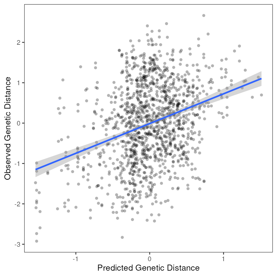
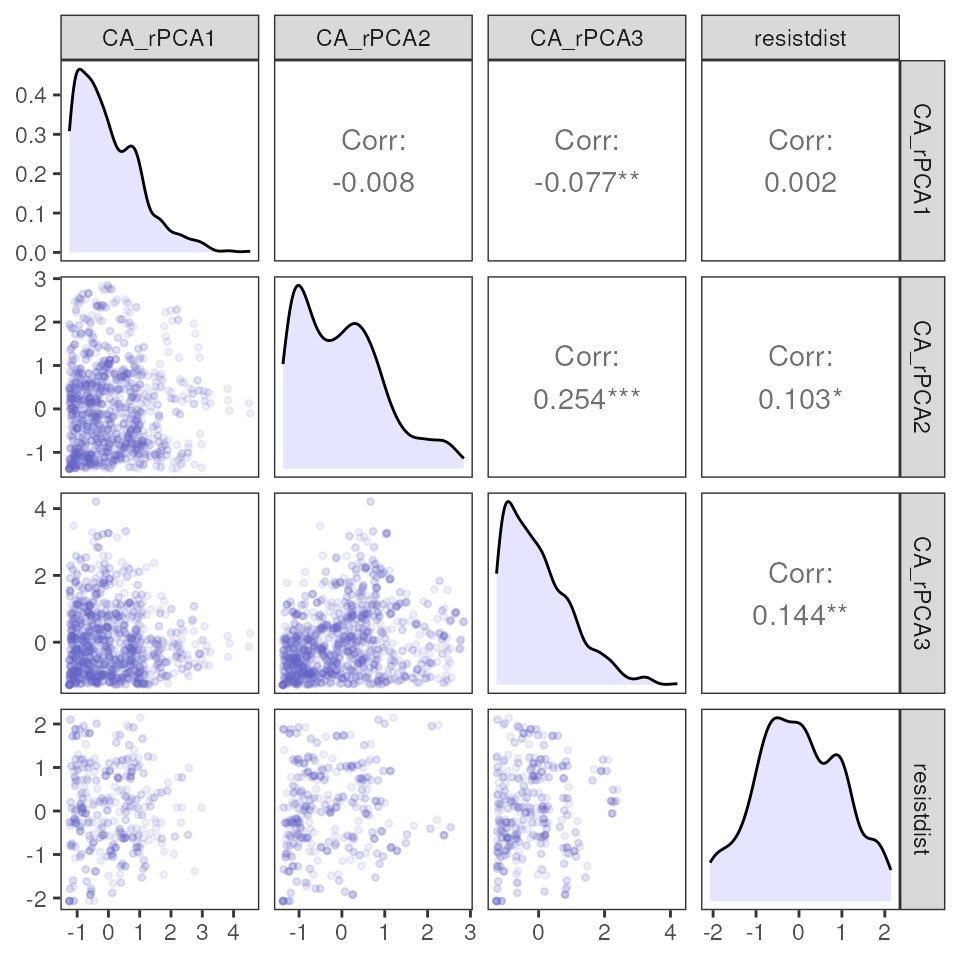
Let’s take a look at the results from our MMRR analyses above. We can
produce several plots to visualize results with the
mmrr_plot() function, including plotting single variable
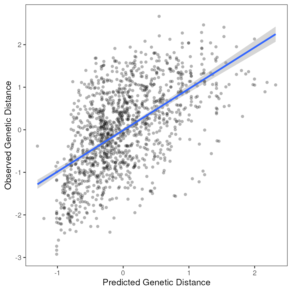
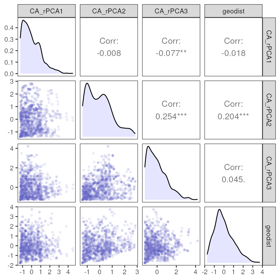
relationships (plot_type = "vars"), plotting the fitted
relationship that compares predicted against the observed genetic
distances (plot_type = "fitted"), or plotting covariances
between the predictor variables (plot_type = "cov").
Lastly, you can set plot_type = "all" to produce all three
of these plots for your MMRR run.
# Single variable plot
mmrr_plot(Y, X, mod = results_full$mod, plot_type = "vars", stdz = TRUE)
# Fitted variable plot
mmrr_plot(Y, X, mod = results_full$mod, plot_type = "fitted", stdz = TRUE)
# Covariance plot
mmrr_plot(Y, X, mod = results_full$mod, plot_type = "cov", stdz = TRUE)
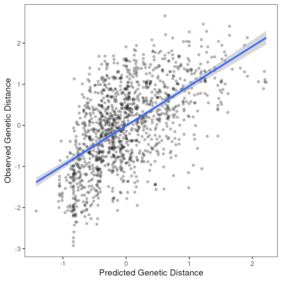
How do the above results compare to those from the “best” model?
mmrr_plot(Y, X, mod = results_best$mod, plot_type = "all", stdz = TRUE)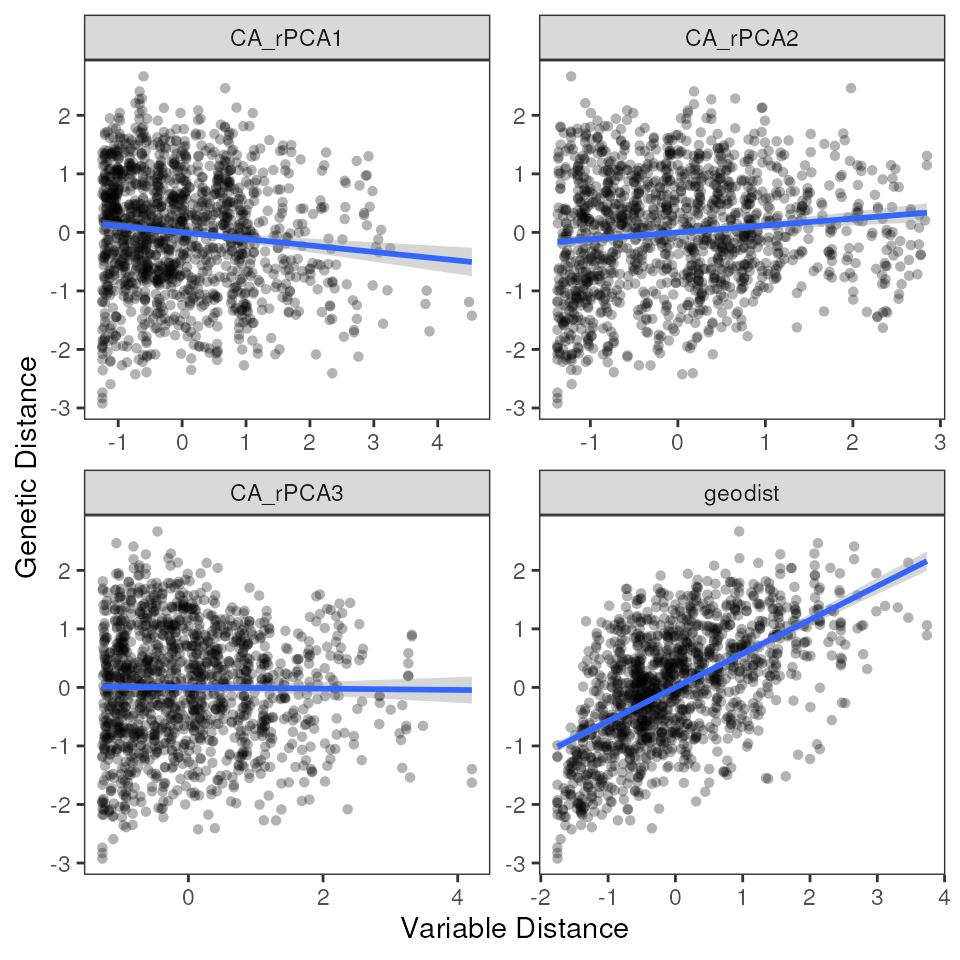
Look at MMRR output statistics with mmrr_table()
We can also take a closer look at the output statistics from our MMRR
runs using the mmrr_table() function. This function will
also provide summary statistics if we set summary_stats to
TRUE (the default). The estimate column contains the coefficients for
each of the variables. N.B.: significance values may change slightly
due to the permutation procedure.
mmrr_table(results_full, digits = 2, summary_stats = TRUE)| var | estimate | p | 95% Lower | 95% Upper |
|---|---|---|---|---|
| CA_rPCA1 | −0.10 | 0.06 | −0.14 | −0.07 |
| CA_rPCA2 | 0.01 | 0.77 | −0.03 | 0.05 |
| CA_rPCA3 | −0.05 | 0.36 | −0.08 | −0.01 |
| geodist | 0.58 | 0.01 | 0.54 | 0.61 |
| Intercept | 0.00 | 0.01 | −0.04 | 0.04 |
| R-Squared: | 0.35 | |||
| F-Statistic: | 181.28 | |||
| F p-value: | 0.01 | |||
Running MMRR with mmrr_do_everything()
The algatr package also has an option to run all of the above
functionality in a single function, mmrr_do_everything().
This function runs MMRR while specifying whether a user would like to
run variable selection or not (using the model argument),
producing a table and all plots automatically. It will automatically
extract environmental variables based on coordinates and calculate
environmental distances from these data. Users can also choose to
include geographic distances within the independent variable matrix by
setting geo = TRUE (the default setting). Please be
aware that the do_everything() functions are meant to be
exploratory. We do not recommend their use for final analyses unless
certain they are properly parameterized.
MMRR with all variables
set.seed(01)
mmrr_full_everything <- mmrr_do_everything(liz_gendist, liz_coords, env = CA_env, geo = TRUE, model = "full")

| var | estimate | p | 95% Lower | 95% Upper |
|---|---|---|---|---|
| CA_rPCA1 | −0.10 | 0.05 | −0.14 | −0.07 |
| CA_rPCA2 | 0.01 | 0.78 | −0.03 | 0.05 |
| CA_rPCA3 | −0.05 | 0.36 | −0.08 | −0.01 |
| geodist | 0.58 | 0.00 | 0.54 | 0.61 |
| Intercept | 0.00 | 0.00 | −0.04 | 0.04 |
| R-Squared: | 0.35 |
|
|
|
| F-Statistic: | 181.28 |
|
|
|
| F p-value: | 0.00 |
|
|
|
Extending MMRR’s functionality with resistance distances
The relationships between geographic distance and/or environmental variables on spatial genetic variation result in patterns of isolation by distance (IBD) or isolation by environment (IBE), respectively. However, one other key phenomenon that can occur - and one in which landscape genomicists are often interested in examining - is one in which landscape features act to restrict gene flow, resulting in a pattern known as isolation by resistance (IBR). IBR is typically investigated by first generating a resistance surface which provides information about how the landscape “resists” gene flow given the study organism. Then, given the resistance surface, resistance distances can be calculated using (once again) a variety of methods, but most typically use circuit theory to model connectivity across the landscape.
The resistance surface can be generated using species distribution models, habitat suitability models, or other types of approaches that simulate forward evolution given sampling localities and genotypes (e.g., resistanceGA; Peterman 2018). Building a reliable resistance surface can be quite complex, requiring many decisions on the part of the researcher and, in some cases, extensive parameterization and model testing to generate this type of surface. These sets of decisions are precisely why algatr does not explicitly implement any IBR methods, but below we describe one way in which the package can be extended to do so.
As was briefly mentioned in the environmental data vignette, the
geo_dist() function is able to calculate resistance-based
distances, largely using the gdistance
package (van
Etten 2017). Importantly, a user must provide a resistance surface
using whichever their preferred method is by specifying the
lyr argument. The function then creates a transition
surface and calculates circuit distances (random-walk commute distances)
using the gdistance::commuteDistance() function.
Although algatr does not have the explicit functionality to quantify
and visualize IBR, we can investigate IBR using MMRR given that this
method conducts a multiple Mantel test given some distance metric. Thus,
it is possible to run geo_dist() specifying
lyr with your resistance raster and use the resulting
distances as input into MMRR. The following is a toy example of
how this could be done. For this example we’ll pretend our resistance
surface is one of our environmental layers (where greater values
indicate more resistance) and use it to calculate our resistance
distances.
# here we aggregate the layer for computational speed
lyr <- aggregate(CA_env$CA_rPCA1, 50)
plot(lyr)
points(liz_coords)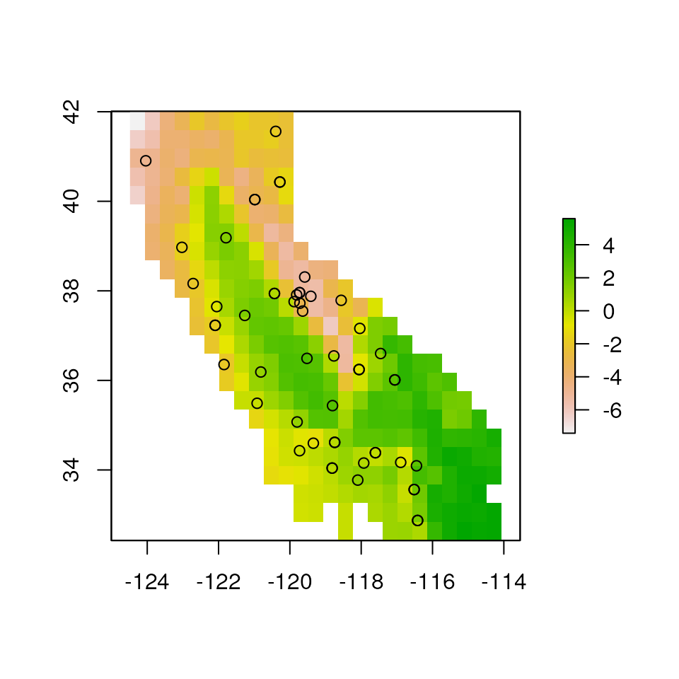
# Recreate MMRR input with resistance distances
# Calculate environmental distances
X <- env_dist(env)
# Add geographic distance to X
X[["resistdist"]] <- geo_dist(liz_coords, type = "resistance", lyr = lyr)
#> Calculating resistance distances... This can be time consuming with many points and large rasters.
Now, we can run MMRR as we did above but including resistance-based distances in our input data.
# Run MMRR with resistance distances
results_resist <- mmrr_run(Y, X, nperm = 99, stdz = TRUE, model = "full")
mmrr_plot(Y, X, mod = results_resist$mod, plot_type = "all", stdz = TRUE)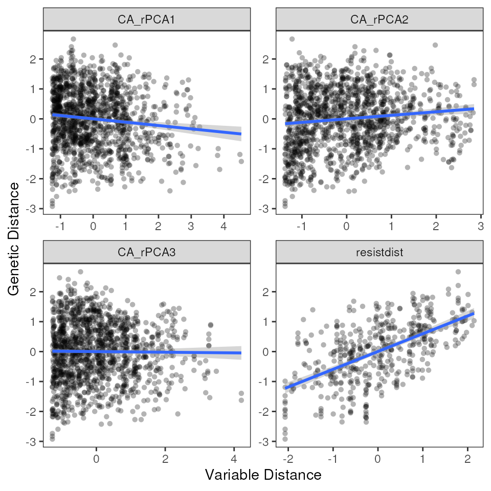
mmrr_table(results_resist)| var | estimate | p | 95% Lower | 95% Upper |
|---|---|---|---|---|
| CA_rPCA1 | −0.05 | 0.39 | −0.12 | 0.02 |
| CA_rPCA2 | 0.20 | 0.01 | 0.12 | 0.28 |
| CA_rPCA3 | 0.12 | 0.15 | 0.05 | 0.20 |
| Intercept | 0.09 | 0.24 | 0.02 | 0.15 |
| resistdist | 0.56 | 0.01 | 0.50 | 0.62 |
| R-Squared: | 0.40 | |||
| F-Statistic: | 76.62 | |||
| F p-value: | 0.01 | |||
Additional documentation and citations
| Citation/URL | Details | |
|---|---|---|
| Manuscript with method | Wang 2013 | Paper describing MMRR method |
| Associated code | MMRR tutorial | Walkthrough of MMRR |