Wingen
wingen_vignette.Rmdwingen
# Install required packages
wingen_packages()If using wingen, please cite the following: Bishop A.P., Chambers E.A., Wang I.J. (2023) Generating continuous maps of genetic diversity using moving windows. Methods in Ecology and Evolution. DOI: https://doi.org/10.1111/2041-210X.14090.
wingen is a package that uses a moving window approach to create continuous maps of genetic diversity. Please see Bishop et al. 2023 for the paper describing the method, and refer to the wingen package for further documentation.
Briefly, wingen takes in genetic data (in the form of a vcf), sampling coordinates, and a raster of a given study area. wingen then moves a window (of a user-specified size) across the landscape, and calculates genetic diversity for any samples that fall within this window. The focal cell (the size of which is determined by the raster layer inputted) is then assigned this resulting genetic diversity value, and the window continues sliding across the landscape. Users are able to specify not only window size, but can also aggregate cells to increase map continuity and decrease computational time, and can perform rarefaction of samples such that uneven sampling does not bias calculations. The resulting wingen map can be smoothed using kriging, and any areas that were undersampled (or fall outside an area of interest, such as a species range, for example) are masked.
There are five key functions within wingen:
preview_gd()provides a reference point for what the window and focal cell look like relative to the landscape; this function also allows users to visualize the sample count in each cell given the parameterswindow_gd()to create a map of genetic diversitykrig_gd()for spatial interpolation (smoothing) of the resulting map using krigingmask_gd()to mask out any undersampled areas (or areas that are not of interest)plot_gd()to plot resulting genetic diversity map andplot_count()to plot the resulting sample count map
Note: Coordinates and rasters used in wingen should be in a projected (planar) coordinate system such that raster cells are of equal sizes. Therefore, spherical systems (including latitude-longitude coordinate systems) should be projected prior to use. An example of how this can be accomplished is shown below. If no CRS is provided, a warning will be given and wingen will assume the data are provided in a projected system. Please refer to the wingen vignette for further information.
Read in and process input data
wingen requires a vcf, sampling coordinates, and a raster layer upon which to move the sliding window across.
load_algatr_example()
#>
#> ---------------- example dataset ----------------
#>
#> Objects loaded:
#> *liz_vcf* vcfR object (1000 loci x 53 samples)
#> *liz_gendist* genetic distance matrix (Plink Distance)
#> *liz_coords* dataframe with x and y coordinates
#> *CA_env* RasterStack with example environmental layers
#>
#> -------------------------------------------------
#>
#>
Coordinates and rasters used in wingen should be in a projected (planar) coordinate system such that raster cells are of equal sizes. Therefore, spherical systems (including latitude-longitude coordinate systems) should be projected prior to use. An example of how this can be accomplished is shown below. If no CRS is provided, a warning will be given. Here we reproject our latitude-longitude coordinates to an equal-area projection for California.
# First, we reformat our dataframe of coordinates into sf coordinates
coords_longlat <- st_as_sf(liz_coords, coords = c("x", "y"), crs = "+proj=longlat")

# Next, the coordinates and raster can be projected to an equal area projection, in this case NAD83 / California Albers (EPSG 3310)
coords_proj <- st_transform(coords_longlat, crs = 3310)
We’ll also want the shape of California for subsequent plotting, so we’ll save one of the environmental PC layers as a SpatRaster object for this purpose and reproject to the same coordinate reference system as the coordinates.
Generate raster layer for sliding window
Although we can use one of the PCs within our CA_env object as a
raster for wingen, the resolution of those layers is unnecessarily high
given our sampling localities, and running wingen (particularly the
kriging step) will take a very long time. To remedy this, we can
generate a raster layer using the coords_to_raster()
function in algatr by providing our sampling coordinates. Using this
function, we can specify the resolution of our raster with the
res argument. Here we choose a very low resolution (i.e.,
large cells) of 50 km to make processing time faster. Note that the
resolution units depend on the coordinate reference system.
liz_lyr <- coords_to_raster(coords_proj, res = 50000, buffer = 5, plot = TRUE)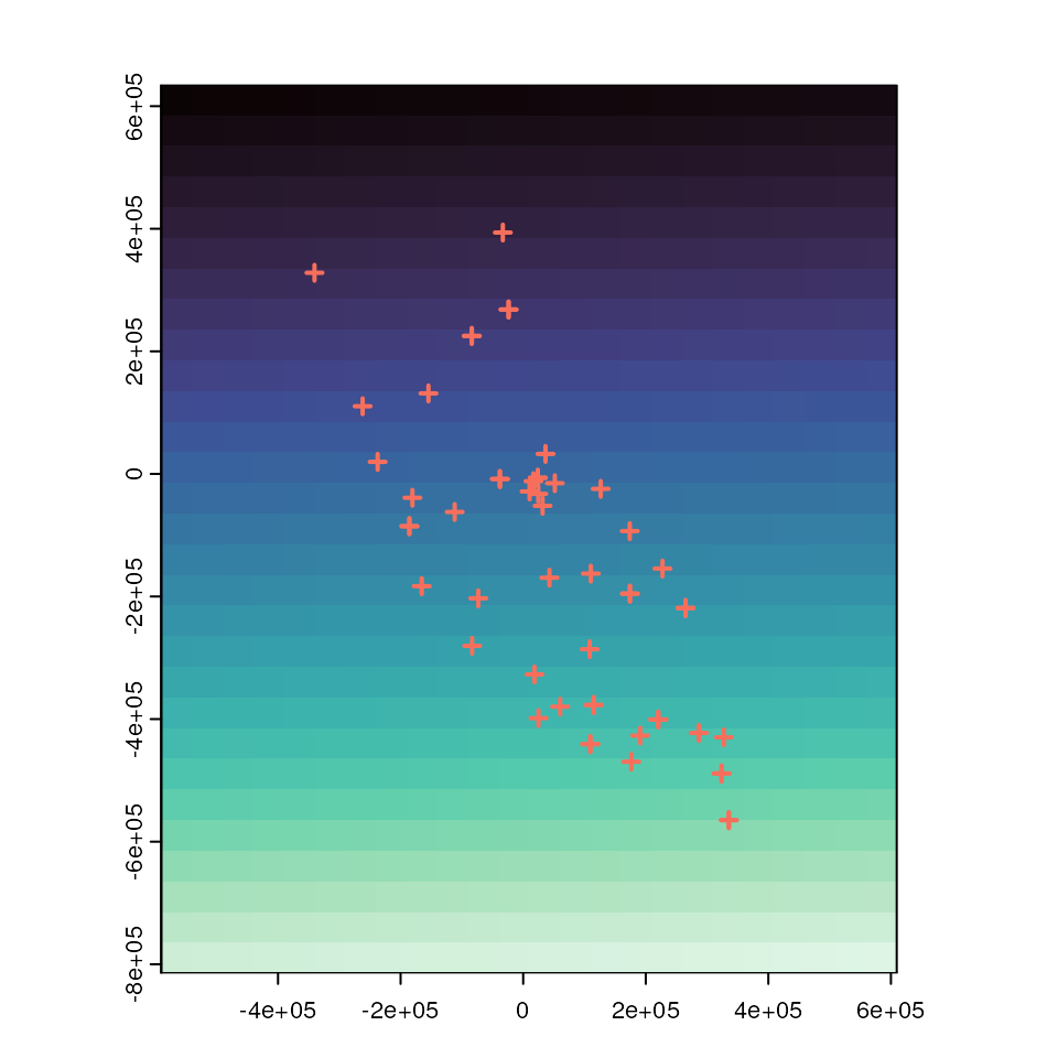
Moving window calculations using preview_gd() and
window_gd()
The window_gd() function takes in a vcf file (the
vcf argument), sampling coordinates (coords
argument), and a RasterLayer for the window to move across (the
lyr argument), and the genetic diversity summary statistic
to calculate (the stat argument); choices are allelic
richness ("allelic.richness" or
"biallelic.richness"), nucleotide diversity
("pi"), or average heterozygosity ("Ho"). For
more options for file types and statistics see the original wingen
vignette.
There are a number of additional arguments within this function, and
the wingen package documentation provides extensive explanations (and
guidelines for testing) these parameters. Briefly, fact
aggregates the input raster layer (by a given factor), wdim
specifies the window dimensions, rarify specifies whether
the user would like samples to be rarified (which then requires users to
specify rarify_n and rarify_nit), and finally
parallel specifies whether you would like to
parallelize.
Preview the moving window
First, we can get an idea of what the size of the cell and moving
window look like using the preview_gd() function. We want
adjust the window size (using the wdim argument) to ensure
(to some extent) that our window size is capturing samples as it slides
across the landscape. Ideally, wdim should be set with the
study system in mind (e.g., the dispersal distance or neighborhood size
of the species). We will also specify that genetic diversity only be
calculated for windows that contain at least two samples
(min_n). This function produces a plot that allows us to
visualize the size of our window compared to the raster layer and
sampling coordinates. The function also returns a sample count raster
map where the value of each cell is how many samples will be included in
each cell’s calculation (to stop this raster from being produced set
sample_count = FALSE).
sample_count <- preview_gd(liz_lyr, coords_proj, wdim = 3, fact = 0)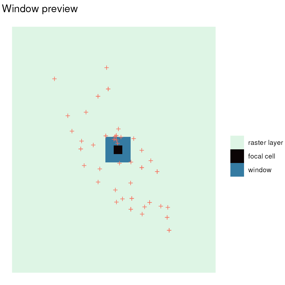
# Visualize the sample count layer
ggplot_count(sample_count)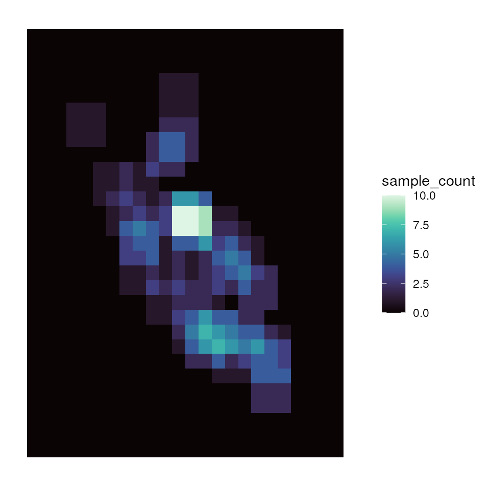
Run the moving window
Next, let’s run the moving window function (window_gd())
using the parameters specified above, calculating nucleotide diversity
(stat = "pi") as our diversity metric. For simplicity’s
sake, we will not perform rarefaction of our samples
(rarify = FALSE, which is the default).
wgd <- window_gd(liz_vcf,
  coords_proj,
  liz_lyr,
  stat = "pi",
  wdim = 3,
  fact = 0
)
#> Loading required namespace: vcfR
#> Loading required namespace: adegenet
Visualizing wingen results
Plot wingen results with ggplot_gd() and
ggplot_count()
wingen allows for plotting maps in two ways: ggplot_gd()
plots the genetic diversity layer, while ggplot_count()
plots the sample count layer. We can also provide a background map using
the bkg argument. You can produce base R plots using
plot_gd() and plot_count()
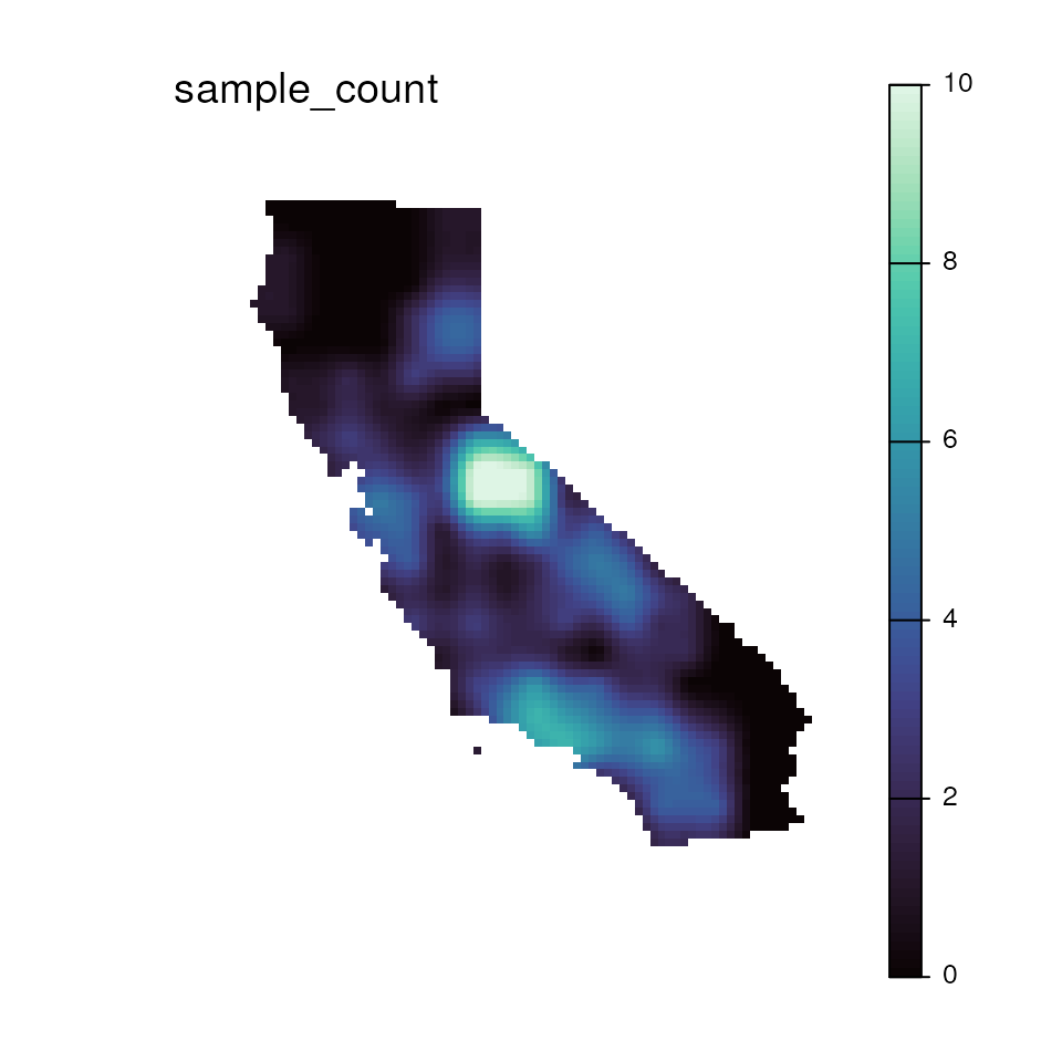
# Plot sample count map
ggplot_count(wgd) + ggtitle("Sample count")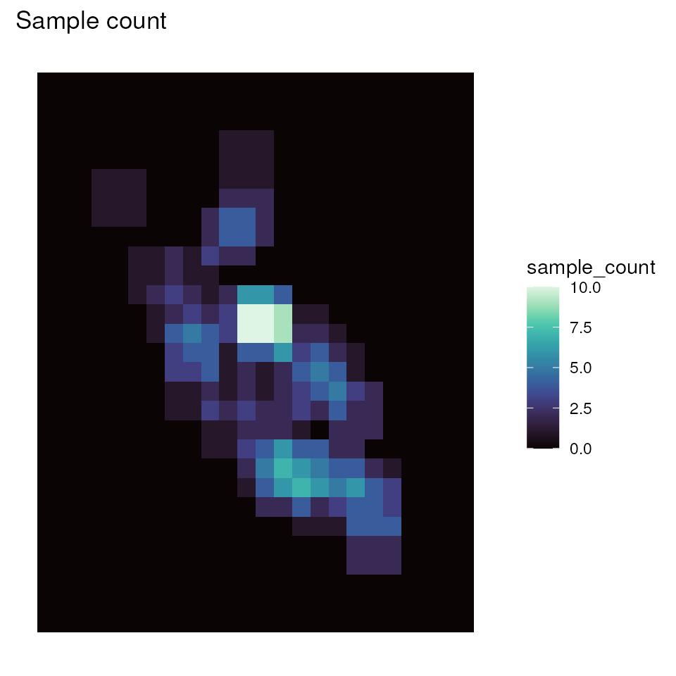
Krige results
Kriging is a type of spatial interpolation that uses a spatial model
to provide estimates of genetic diversity from unsampled locations; in
the cae of wingen, it also allows for smoother maps of genetic
diversity. We can krige our moving window map using the
krig_gd() function by providing the results from the moving
window, and a raster layer upon which kriging is performed (an
“interpolation grid”); if no interpolation grid is provided, kriging
will be done on the moving window layer. The index argument
specifies which layer we want to krige across; in our case, we’ll krige
both layers 1 (genetic diversity) and 2 (sample counts) of the wgd
object because we will eventually want to visualize both kriged maps.
Kriging can be computationally intensive, but we can remedy this by
aggregating the raster layer upon which kriging is performed using
either the agg_r or agg_grd arguments
depending on whether we want to aggregate across the moving window layer
or the interpolation grid layer, respectively. In our case, given the
resolution of lyr, we want to disaggregate by a factor of 5
to get a smoother interpolated surface, so we’ll set
disagg_grd = 5. If only the moving window layer is provided
for kriging, we can use the disagg_r argument to set this
parameter.
The resulting object, kgd, is a RasterStack object
containing two layers: our genetic diversity statistic (pi), and our
sample count information (sample_count).
kgd <- krig_gd(wgd, index = 1:2, liz_lyr, disagg_grd = 5)
#> [using ordinary kriging]
#> [using ordinary kriging]
summary(kgd)
#> pi sample_count
#> Min. :0.02683 Min. : 0.0000
#> 1st Qu.:0.06456 1st Qu.: 0.0000
#> Median :0.06497 Median : 0.0000
#> Mean :0.06497 Mean : 0.6904
#> 3rd Qu.:0.06499 3rd Qu.: 0.6261
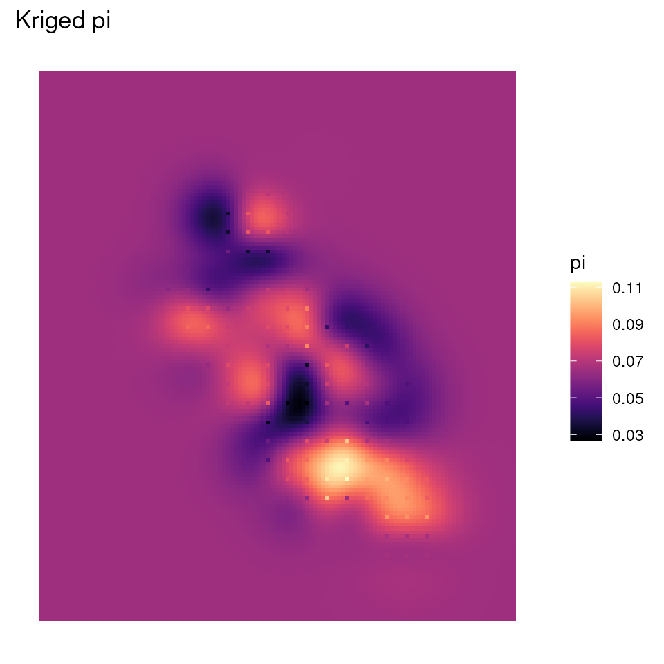
#> Max. :0.11302 Max. :10.0000Let’s look at the plots for the kriged results, and let’s avoid
including the background shape for now (i.e., no bkg
argument). Note that the overall shape of this kriged map is rectangular
because of the lyr raster shape.
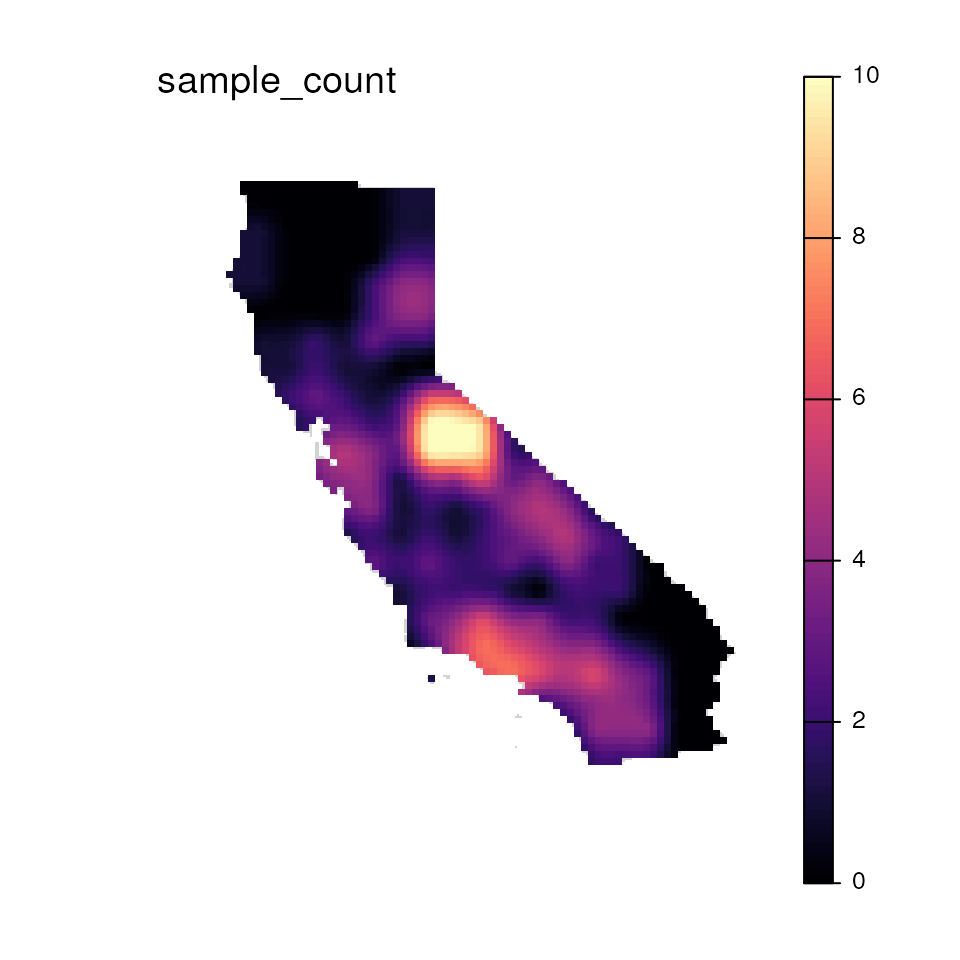
# Plot kriged sample count map
ggplot_count(kgd) + ggtitle("Kriged sample counts")
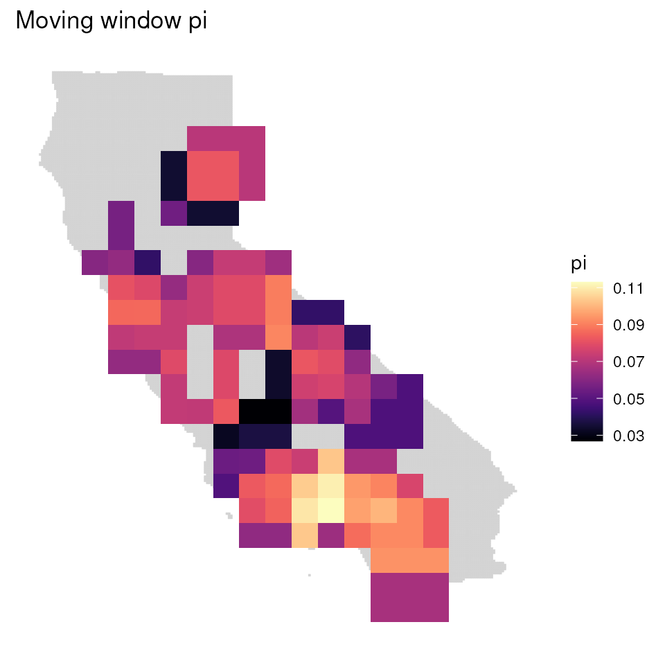
Mask using sample counts
Finally, we may want to mask out any areas that we’re not interested
in using the mask_gd() function. wingen provides several
ways to perform masking, but we will focus on two for this vignette. The
mask_gd() function is quite simple in that it takes in the
layer you want masked (kgd, in our case) and the layer you
want to mask to. Let’s first mask areas based on sample count. Recall
that above, we called krig_gd() using indices 1 and 2,
which told wingen to krige on both the genetic diversity (pi) and sample
count layers. We’ll make use of the kriged sample count layer now by
masking according to it. The minval argument specifies the
minimum value below which areas will be masked, meaning that any areas
that do not contain any samples will be masked. Let’s compare two maps
masked in this way with differing minval values.
As you can see, more areas are masked as we increase
minval.
mgd_1 <- mask_gd(kgd, kgd[["sample_count"]], minval = 1)
mgd_2 <- mask_gd(kgd, kgd[["sample_count"]], minval = 2)

ggplot_gd(mgd_1, bkg = envlayer) + ggtitle("Kriged & masked pi")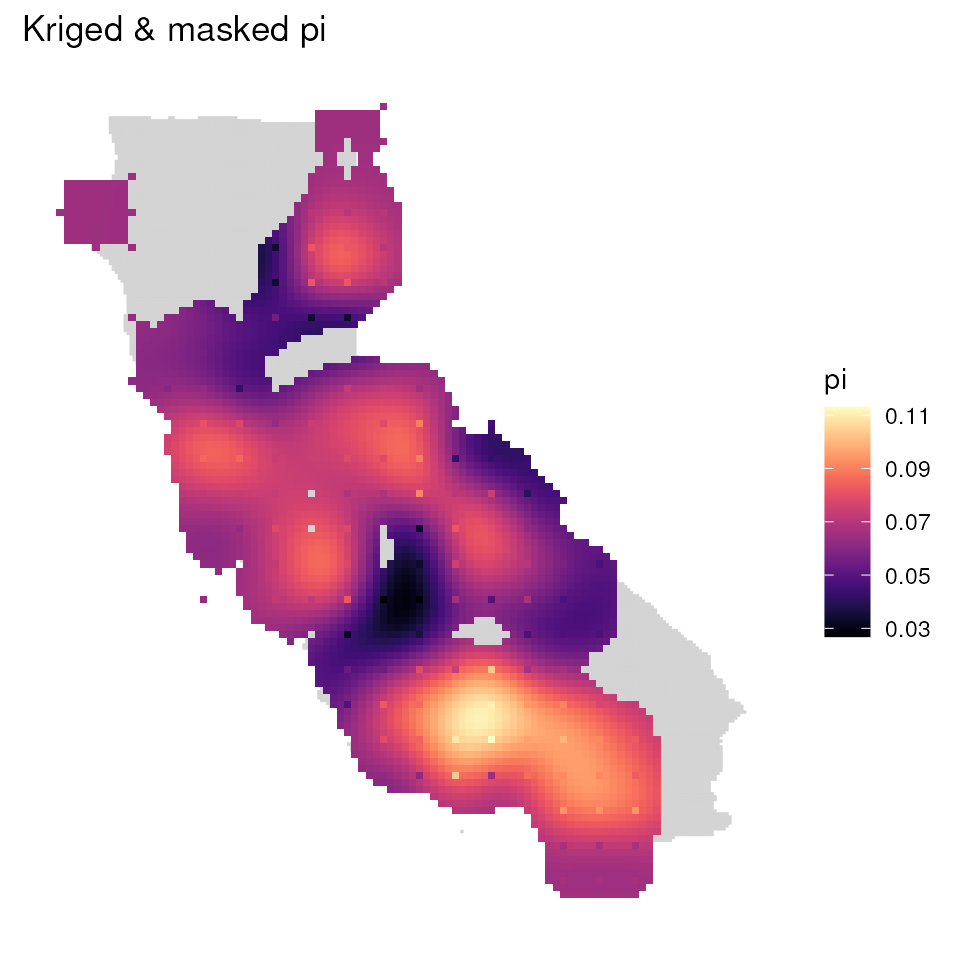
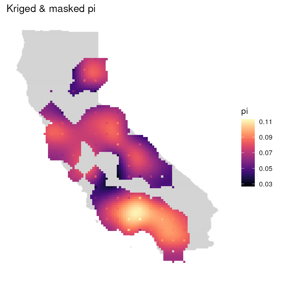
Mask using state boundaries
Next, let’s mask out any areas outside of California state boundaries
using our envlayer object.
One thing to keep in mind is that if you are masking using a raster,
you need to ensure that pixels match between the object to be masked and
the object to use as a mask. If they aren’t the same, or if their
extents are different, you will either get an error or the map will look
wonky. To remedy this, we can use terra’s resample()
function. This function will resample a raster (here,
envlayer) based on an inputted raster (here,
mgd_1).
# Resample envlayer based on masked layer
r <- terra::resample(envlayer, mgd_1)

# Perform masking
mgd <- mask_gd(mgd_1, r)

# Plot masked map
ggplot_gd(mgd, bkg = envlayer) + ggtitle("Kriged & masked pi")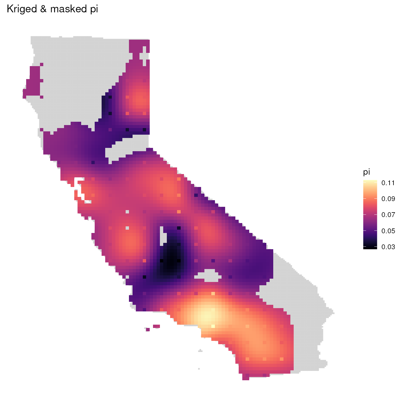
Running wingen with wingen_do_everything()
The algatr package also has an option to run all of the above
functionality in a single function, wingen_do_everything().
If you want to take a look at the preview first, you can set
preview = TRUE; to krige, set kriged = TRUE,
and to mask, set masked = TRUE. If preview is
set to TRUE, the preview plot will be printed and a user can enter into
the console whether they would like to continue the wingen run with
existing parameter settings, or else halt the run. Please be
aware that the do_everything() functions are meant to be
exploratory. We do not recommend their use for final analyses unless
certain they are properly parameterized.
WARNING: Many wingen arguments are excluded from
wingen_do_everything() to reduce the number of arguments in
the function. Thus, we strongly advise against using this function for
actual analyses and encourage users to explore and test the individual
wingen functions given their datasets.
Below, we’ll run wingen with the following:
No preview generated before running wingen (
preview = FALSE)Window size of 3x3 (
wdim = 3), no aggregation factor for moving window (fact = 0)Pi as our genetic diversity statistic (
stat = "pi"); this is also the defaultNo rarefaction (
rarify = FALSE)Kriging (of both genetic diversity and sample count layers;
kriged = TRUEandindex = 1:2) with a disaggregation factor of 4 for kriging (disagg_grd = 4)Masking to California state boundaries (
mask = envlayer)Plot kriged and masked sample count (
plot_count = TRUE)
results <- wingen_do_everything(
  gen = liz_vcf,
  lyr = liz_lyr,
  coords = coords_proj,
  wdim = 3,
  fact = 0,
  sample_count = TRUE,
  preview = FALSE,
  min_n = 2,
  stat = "pi",
  rarify = FALSE,
  kriged = TRUE,
  grd = liz_lyr,
  index = 1:2,
  agg_grd = NULL, disagg_grd = 4,
  agg_r = NULL, disagg_r = NULL,
  masked = TRUE, mask = envlayer,
  bkg = envlayer, plot_count = TRUE
)
#> Please be aware: the do_everything functions are meant to be exploratory. We do not recommend their use for final analyses unless certain they are properly parameterized.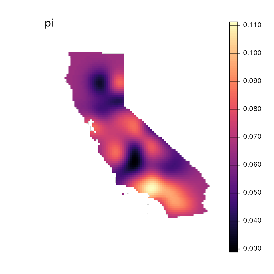
Additional documentation and citations
| Citation/URL | Details | |
|---|---|---|
| Manuscript with method | Bishop et al. 2023 | Paper describing wingen methodology and package |
| R package documentation | Available on Github | Code, vignette |
Retrieve wingen’s vignette:
# vignette("wingen-vignette")