Genetic distances
gen_dist_vignette.RmdCalculating genetic distances
# Install required packages
gen_dist_packages()For several landscape genomics analyses, a pairwise genetic distance
matrix is required as input. There are a variety of ways to calculate
genetic distance, and the main function in this package,
gen_dist(), allows a user to choose from five different
genetic distances and saves square distance matrices as csv files. The
five genetic distance metrics are specified using the
dist_type argument and are as follows:
Euclidean distance (the
"euclidean"argument), which uses thedistance()function within the ecodist packageBray-Curtis distance (the
"bray_curtis"argument), which uses thedistance()function within the ecodist packageProportion of shared alleles (the
"dps"argument), which uses thepropShared()function within the adegenet packagePC-based distance (the
"pc"argument), which uses theprcomp()function within the stats package and selects the number of PCs using a Tracy-Widom test (ifnpc_selection = "auto"; also requires specifyingcriticalpoint[see below for details]) or user-inputted PCs based on examining a screeplot and manually entering a value into the console (ifnpc_selection = "manual")Processing distances generated using Plink (the
"plink"argument). This type of distance requires providing paths to two plink output files (the distance file,plink_file, and the ID file,plink_id_file); the distance file must be a square (i.e., symmetric) distance matrix
A good place to start to understand these metrics is Shirk et al., 2017, who tested a number of different genetic distance metrics (including most of the above) and compared results for use in landscape genetics analyses.
This package also allows a user to look at the relationship between
distance metrics using the gen_dist_corr() function, and to
visualize genetic distance matrices with a heatmap using the
gen_dist_hm() function.
Load example dataset
load_algatr_example()
#>
#> ---------------- example dataset ----------------
#>
#> Objects loaded:
#> *liz_vcf* vcfR object (1000 loci x 53 samples)
#> *liz_gendist* genetic distance matrix (Plink Distance)
#> *liz_coords* dataframe with x and y coordinates
#> *CA_env* RasterStack with example environmental layers
#>
#> -------------------------------------------------
#>
#>
Calculate genetic distances with gen_dist()
Euclidean, Bray-Curtis, and PC-based genetic distance metrics
require no missing data. A simple imputation
(to the median or mean, depending on the distance metric) is built into
the gen_dist() function mostly for creating test datasets;
we highly discourage using this form of
imputation in any of your analyses. You can take a look at the
str_impute() function description in the data processing
vignette for information on an alternate imputation method provided in
algatr.
To calculate Euclidean distances between our samples:
# Calculate Euclidean distance matrix
euc_dists <- gen_dist(liz_vcf, dist_type = "euclidean")
#> Loading required namespace: vcfR
#> Loading required namespace: adegenet
#> Warning in gen_dist(liz_vcf, dist_type = "euclidean"): NAs found in genetic
#> data, imputing to the median (NOTE: this simplified imputation approach is
#> strongly discouraged. Consider using another method of removing missing data)

euc_dists[1:5, 1:5]
#>            ALT3   BAR360     BLL5     BNT5     BOF1
#> ALT3    0.00000 22.92379 17.26992 21.08910 18.77498
#> BAR360 22.92379  0.00000 17.85357 19.50000 17.56417
#> BLL5   17.26992 17.85357  0.00000 15.76388 12.63922
#> BNT5   21.08910 19.50000 15.76388  0.00000 15.99219
#> BOF1   18.77498 17.56417 12.63922 15.99219  0.00000
Now, let’s process Plink distances, keeping in mind that the provided Plink distance matrix must be square (i.e., symmetric). Refer the Plink documentation for how to generate a square distance matrix.
plink_dists <- gen_dist(plink_file = system.file("extdata", "liz_test.dist", package = "algatr"), plink_id_file = system.file("extdata", "liz_test.dist.id", package = "algatr"), dist_type = "plink")
#> Rows: 53 Columns: 53
#> ── Column specification ────────────────────────────────────────────────────────
#> Delimiter: "\t"
#> dbl (53): X1, X2, X3, X4, X5, X6, X7, X8, X9, X10, X11, X12, X13, X14, X15, ...
#>
#> ℹ Use `spec()` to retrieve the full column specification for this data.
#> ℹ Specify the column types or set `show_col_types = FALSE` to quiet this message.
#> Rows: 53 Columns: 2
#> ── Column specification ────────────────────────────────────────────────────────
#> Delimiter: "\t"
#> chr (2): X1, X2
#>
#> ℹ Use `spec()` to retrieve the full column specification for this data.
#> ℹ Specify the column types or set `show_col_types = FALSE` to quiet this message.
Finally, let’s calculate PC-based distances. There are two options
for selecting the “best” number of PCs, specified using the
npc_selection argument: "auto", which runs a
Tracy-Widom test and selects the number of significant eigenvalues of
the PC, or "manual", in which a screeplot is printed to the
screen and a user can manually enter the number of PCs to choose into
the console. For the automatic option, a significance threshold must be
specified using the criticalpoint argument; significance
levels of 0.05, 0.01, 0.005, or 0.001 correspond to the
criticalpoint argument being 0.9793, 2.0234, 2.4224, or
3.2724, respectively).
pc_dists <- gen_dist(liz_vcf, dist_type = "pc", npc_selection = "auto", criticalpoint = 2.0234)
#> Warning in gen_dist(liz_vcf, dist_type = "pc", npc_selection = "auto",
#> criticalpoint = 2.0234): NAs found in genetic data, imputing to the median
#> (NOTE: this simplified imputation approach is strongly discouraged. Consider
#> using another method of removing missing data)
Compare genetic distance results
Plot comparisons between two genetic distances with
gen_dist_corr()
To compare between the genetic distances you just produced, we can plot them:
# Plot some pairwise comparisons, providing names for the metrics
p_euc_plink <- gen_dist_corr(euc_dists, plink_dists, "Euclidean", "Plink")
#> Joining with `by = join_by(comparison, name)`
#> Warning: `aes_string()` was deprecated in ggplot2 3.0.0.
#> ℹ Please use tidy evaluation idioms with `aes()`.
#> ℹ See also `vignette("ggplot2-in-packages")` for more information.
#> ℹ The deprecated feature was likely used in the algatr package.
#>   Please report the issue to the authors.
#> This warning is displayed once per session.
#> Call `lifecycle::last_lifecycle_warnings()` to see where this warning was
#> generated.
p_pc_plink <- gen_dist_corr(pc_dists, plink_dists, "PC_based", "Plink")
#> Joining with `by = join_by(comparison, name)`

# Show all plots as panels on a single plot
plot_grid(p_euc_plink, p_pc_plink, nrow = 1)
#> Warning: Removed 1378 rows containing missing values or values outside the scale range
#> (`geom_point()`).
#> Warning: Removed 1378 rows containing missing values or values outside the scale range
#> (`geom_point()`).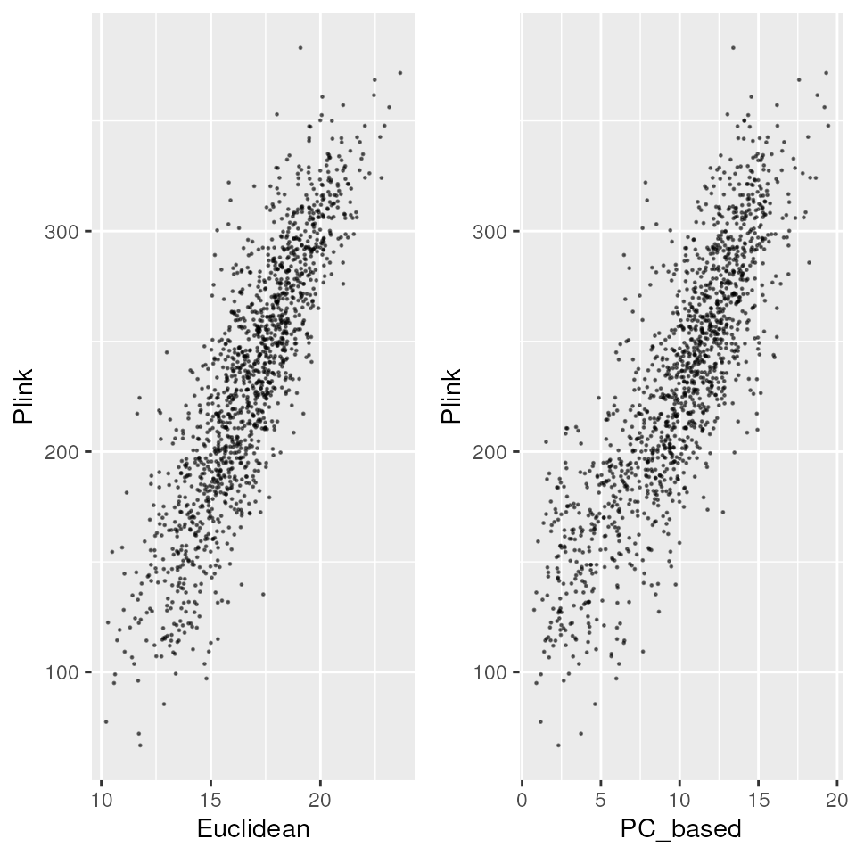
Plot heatmap of one of the genetic distances with
gen_dist_hm()
Let’s look at a heatmap of Euclidean distance for our example dataset.
gen_dist_hm(euc_dists)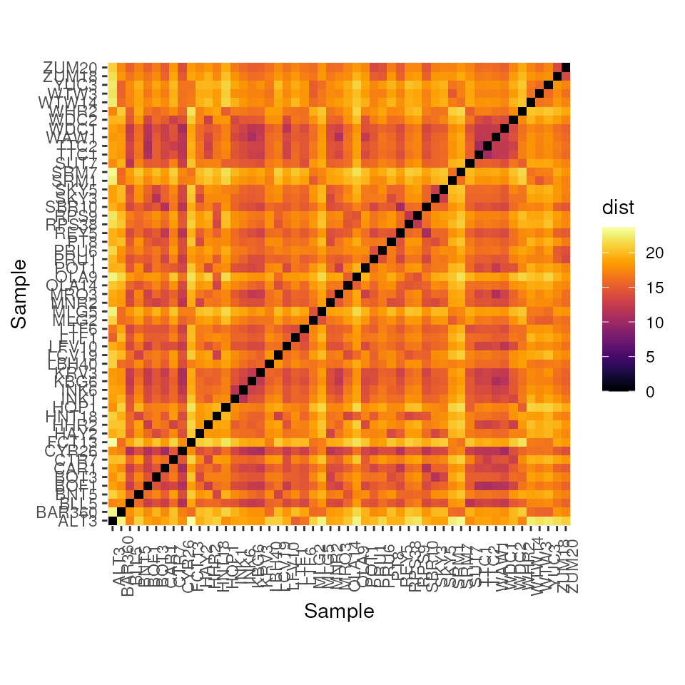
Let’s look at a heatmap of the DPS measure of genetic distance which
is calculated as 1 - proportion of shared alleles:
dps_dists <- gen_dist(liz_vcf, dist_type = "dps")
#> Warning: Prior to May 2025, this function incorrectly returned the proportion
#> of shared alleles (PS) instead of the genetic distance measure: DPS = 1 - PS.
#> Please review results from prior versions accordingly. This warning will appear
#> once per session. To suppress, set options(wingen.quiet_dps_warning = TRUE).
gen_dist_hm(dps_dists)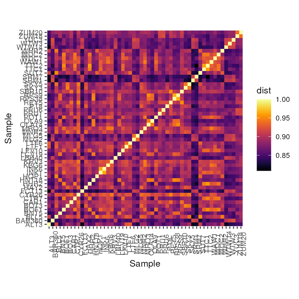
Additional documentation and citations
| Citation/URL | Details | |
|---|---|---|
| Associated code | Goslee & Urban 2007 | algatr’s calculation of Euclidean and Bray-Curtis distances using
the distance() function within the ecodist package |
| Associated code | Jombart 2008; Jombart & Ahmed 2011 | algatr’s calculation of proportion of shared alleles using the
propShared() function within the adegenet package |
| Associated literature | Shirk et al., 2017 | Paper testing a number of different genetic distance metrics (including those used by algatr) for landscape genomics |