Environmental data processing
enviro_data_vignette.RmdProcessing environmental data for landscape genomics
# Install required packages
envirodata_packages()
library(terra)
library(raster)
library(RStoolbox)
library(ggplot2)
library(geodata)
library(viridis)
library(wingen)
library(tidyr)
library(tibble)
For landscape genomic analyses, environmental data layers must be processed in several ways before they can be used as input into methods. This vignette will explore several ways to process environmental data:
get_worldclim()to pull environmental layers remotely from the WorldClim database-
Detect collinearity:
check_env()to detect collinearity between environmental layerscheck_vals()to detect collinearity between extracted environmental valuescheck_dists()to detect collinearity between geographic and environmental distances
rasterPCA()to perform a raster PCA on a stack of environmental layers to reduce dimensionalitycoords_to_raster()to create a raster layer from coordinate data (using the wingen package)env_dist()to calculate environmental distancesgeo_dist()to calculate geographic distances between coordinates
Load example data
load_algatr_example()
#>
#> ---------------- example dataset ----------------
#>
#> Objects loaded:
#> *liz_vcf* vcfR object (1000 loci x 53 samples)
#> *liz_gendist* genetic distance matrix (Plink Distance)
#> *liz_coords* dataframe with x and y coordinates
#> *CA_env* RasterStack with example environmental layers
#>
#> -------------------------------------------------
#>
#>
Introduction to environmental data files and object types
Briefly, in R, any (geo)spatial data can be represented using points, vectors, or rasters. Points represent coordinates. Vectors are used for discrete phenomena that have clear boundaries (e.g., a country), while rasters are used to represent continuous data (e.g., precipitation). Rasters are able to represent continuous data by dividing up the landscape into a grid of equally sized cells; each cell is then assigned one (or more) values for relevant variables. In our case, taking California as an example, points represent sampling coordinates, vectors represent polygons (e.g., the state of California), and rasters store different environmental layers (e.g. temperature, precipitation) for California.
There are two main packages algatr uses to process and manipulate environmental data: terra (Hijmans 2022) and raster (Hijmans 2022). Both of these packages have excellent resources and walkthroughs (see here for terra; see here for raster) that explain in depth environmental data processing and manipulation in R.
Each of these packages has their own classes to represent rasters.
Within the terra package, the SpatRaster class is used to
represent rasters, while the raster package uses
RasterLayer (single-layer raster data),
RasterBrick and RasterStack (both are
multi-variable raster data but differ in how many files can be linked to
them) classes. No matter which class is used to represent rasters, the
fundamental parameters that describe these rasters are always the same:
numbers of rows, columns, the spatial extent, and the coordinate
reference system (CRS) for proper projection.
Ensuring that the CRS between your coordinates and raster layer is particularly important. For all of algatr’s methods, if no CRS is provided, a warning will be generated but the respective method will run assuming that the coordinates and raster CRS match; if the CRS between these two inputs do not match, algatr will throw an error. Also keep in mind that some methods cannot be performed with non-projected data (such as kriging), so users must always transform their coordinates if they’re in lat/long, for example. Refer to the wingen vignette (here) for further information how to convert lat/long coordinates to a projected system.
Gather environmental data using get_worldclim()
WorldClim is a database that provides environmental layers for the
entire globe (excluding Antarctica); the data contained are four monthly
variables and 18 bioclimatic variables, which are provided in tiles. The
get_worldclim() function retrieves and extracts WorldClim
data (using the worldclim_tile() function in the geodata
package) from relevant tiles based on your sampling coordinates, drawing
a convex hull shape to connect all data points.
Users can add a buffer around sampling coordinates using the
buff argument, which corresponds to the proportion of the
spatial extent for the coordinates. Tile size (i.e., spatial resolution)
is specified using the res argument, which corresponds to
arc-minutes. The default is the 30s dataset (0.5 arc-mins), with a
buffer of 0.01.
Because get_worldclim can take some time, the following
code will not knit within the vignette but will give you an idea of how
to run the function with the example data.
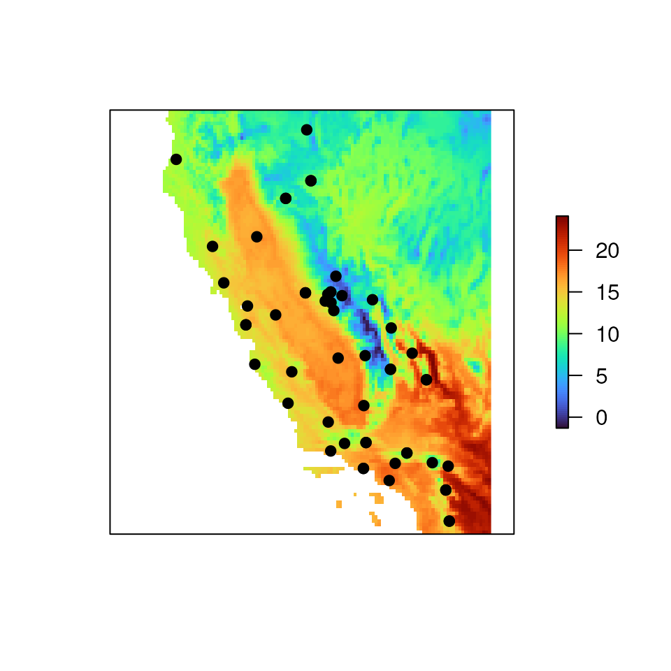
wclim <- get_worldclim(coords = liz_coords, res = 5) # can set save_output = TRUE if you want a directory with files madeNotice that wclim is a terra SpatRaster
object. Let’s take a look at what this object looks like.
# Load wclim object
data("wclim")
# Look at one of the layers, which corresponds to tile_15_wc2.1_30s_bio_1
wclim[[1]]
#> class      : RasterLayer
#> dimensions : 113, 120, 13560  (nrow, ncol, ncell)
#> resolution : 0.08333333, 0.08333333  (x, y)
#> extent     : -125.25, -115.25, 32.58333, 42  (xmin, xmax, ymin, ymax)
#> crs        : +proj=longlat +datum=WGS84 +no_defs
#> source     : memory
#> names      : bio1
#> values     : -1.311542, 24.08433  (min, max)
Now, let’s plot one of the variables and overlay our sampling coordinates on top.
Detecting collinearity
An important first check for any landscape genomics analysis is to
detect collinearity between sets of variables. Specifically, we always
want to verify that there is no collinearity (within a given threshold)
between environmental layers (using check_env()), extracted
values from environmental layers (using check_vals()), and
geographic and environmental distances (using
check_dists()) as many of the methods used for landscape
genomics assume that these variables are independent.
Collinearity among environmental layers
The check_env() function calculates the Pearson
correlation coefficient for pairwise comparisons of environmental
layers. The threshold is the correlation coefficient; it
defaults to 0.7. The output from this function is a list containing (1)
a dataframe of correlated environmental pairs that fall above the
threshold, and (2) a correlation matrix with all pairwise correlation
coefficients.
cors_env <- check_env(wclim)
#> Warning: The extracted values for 19 pairs of variables had correlation coefficients > 0.7. algatr recommends reducing collinearity by removing correlated variables or performing a PCA before proceeeding.
# There are many pairs of layers that have correlation coefficients > 0.7 (the default threshold)
# For the sake of argument, we can also run this function on the CA_env object:
check_env(CA_env)
#> $cor_df
#> [1] var1 var2 r
#> <0 rows> (or 0-length row.names)
#>
#> $cor_matrix
#>              CA_rPCA1     CA_rPCA2     CA_rPCA3
#> CA_rPCA1 1.000000e+00 2.367727e-11 4.231118e-11
#> CA_rPCA2 2.367727e-11 1.000000e+00 3.888803e-11
#> CA_rPCA3 4.231118e-11 3.888803e-11 1.000000e+00
# None of the pairwise comparisons exceed the threshold value
Collinearity among extracted environmental values
Similar to the above, the check_vals() function
determines collinearity using Pearson’s correlation coefficients, but it
does so on extracted environmental variables at each of the sampling
coordinates. This will also generate a plot showing the pairwise
correlations between environmental variables.
# Once again, we can see that there are many pairs of variables that exceed the threshold
check_result <- check_vals(wclim, liz_coords)
#> Warning in crs_check(coords, envlayers): No CRS found for the provided
#> coordinates. Make sure the coordinates and the raster have the same projection
#> (see function details or vignette)
#> Warning: The extracted values for 25 pairs of variables had correlation coefficients > 0.7. algatr recommends reducing collinearity by removing correlated variables or performing a PCA before proceeeding.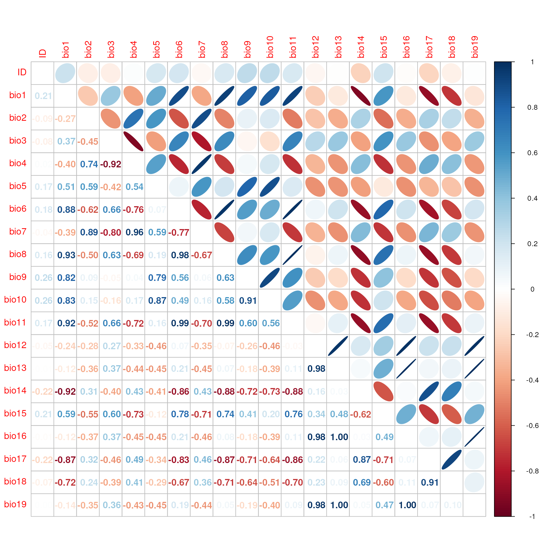
head(check_result$cor_df)
#>   var1 var2         r
#> 1 bio2 bio4 0.7363230
#> 2 bio1 bio6 0.8829763
#> 3 bio2 bio7 0.8851769
#> 4 bio4 bio7 0.9640441
#> 5 bio1 bio8 0.9317171
#> 6 bio6 bio8 0.9761442
# Check using the CA_env object; note that these values are quite different from those from check_env()
check_vals(CA_env, liz_coords)
#> Warning in crs_check(coords, envlayers): No CRS found for the provided
#> coordinates. Make sure the coordinates and the raster have the same projection
#> (see function details or vignette)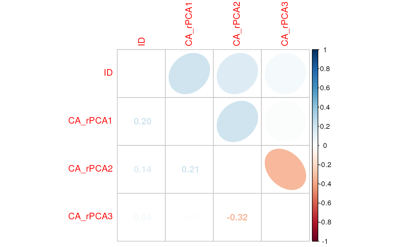
#> $cor_df
#> [1] var1 var2 r
#> <0 rows> (or 0-length row.names)
#>
#> $cor_matrix
#>                  ID   CA_rPCA1   CA_rPCA2    CA_rPCA3
#> ID       1.00000000 0.20306375  0.1439392  0.04309331
#> CA_rPCA1 0.20306375 1.00000000  0.2095724  0.01194543
#> CA_rPCA2 0.14393920 0.20957242  1.0000000 -0.32015438
#> CA_rPCA3 0.04309331 0.01194543 -0.3201544  1.00000000
Collinearity between distances
The check_dists() function determines collinearity
between geographic and environmental distances. It does so by extracting
values at sampling coordinates, and then calculating geographic and
environmental distances and runs a Mantel test on resulting distances.
Environmental distances are calculated using Euclidean distances, while
geographic distances can be Euclidean, topographic, or resistance
distances, though the default is Euclidean. The result of this function
is to output the p-value and Mantel’s r and indicate which distances are
significantly correlated.
check_results <- check_dists(wclim, liz_coords)
#> Warning in crs_check(coords, envlayers): No CRS found for the provided
#> coordinates. Make sure the coordinates and the raster have the same projection
#> (see function details or vignette)
#> Warning: The distances for 121 pairs of variables are significantly correlated. algatr recommends reducing collinearity by removing correlated variables or performing a PCA before proceeeding.
head(check_results$mantel_df)
#>   var1 var2    p         r
#> 1  geo bio2 0.02 0.1465585
#> 2  geo bio3 0.02 0.1153701
#> 3 bio2 bio3 0.01 0.3687943
#> 4  geo bio4 0.01 0.1660475
#> 5 bio2 bio4 0.01 0.5724731
#> 6 bio3 bio4 0.01 0.8417016
# We can see that PC2 from CA_env and geo dists are significantly correlated!
check_dists(CA_env, liz_coords)
#> Warning in crs_check(coords, envlayers): No CRS found for the provided
#> coordinates. Make sure the coordinates and the raster have the same projection
#> (see function details or vignette)
#> Warning: The distances for 2 pairs of variables are significantly correlated. algatr recommends reducing collinearity by removing correlated variables or performing a PCA before proceeeding.
#> $mantel_df
#>       var1     var2    p         r
#> 1      geo CA_rPCA2 0.01 0.2037404
#> 2 CA_rPCA2 CA_rPCA3 0.01 0.2544182
#>
#> $p
#>          [,1] [,2] [,3] [,4] [,5]
#> geo        NA 0.08 0.56 0.01 0.28
#> ID         NA   NA 0.74 0.08 0.07
#> CA_rPCA1   NA   NA   NA 0.52 0.82
#> CA_rPCA2   NA   NA   NA   NA 0.01
#> CA_rPCA3   NA   NA   NA   NA   NA
#>
#> $r
#>          [,1]      [,2]        [,3]        [,4]        [,5]
#> geo        NA 0.0724489 -0.01841863  0.20374038  0.04462286
#> ID         NA        NA -0.04253070  0.06336224  0.08223415
#> CA_rPCA1   NA        NA          NA -0.00798325 -0.07707443
#> CA_rPCA2   NA        NA          NA          NA  0.25441819
#> CA_rPCA3   NA        NA          NA          NA          NA
Perform a raster PCA on environmental layers
Because of collinearity issues, and because we may not want to deal
with dozens of environmental layers at a time, we can perform a PCA on
our rasters using the rasterPCA() function in the RStoolbox
package; this function can take in a SpatRaster or
RasterStack object. Let’s use the wclim object
we generated above using the get_worldclim() function,
which contains 19 environmental variables. The result of this function
is a list containing the model information, and a RasterBrick object
containing multiple layers of PCA scores. One can also use the
nComp argument to only extract the top n PCs; in many
cases, the top three PCs may explain the majority of the variance of the
data, and so only those will be considered for further analyses.
env_pcs <- rasterPCA(wclim, spca = TRUE)

# Let's take a look at the results for the top three PCs
plots <- lapply(1:3, function(x) ggR(env_pcs$map, x, geom_raster = TRUE))

plots[[1]] 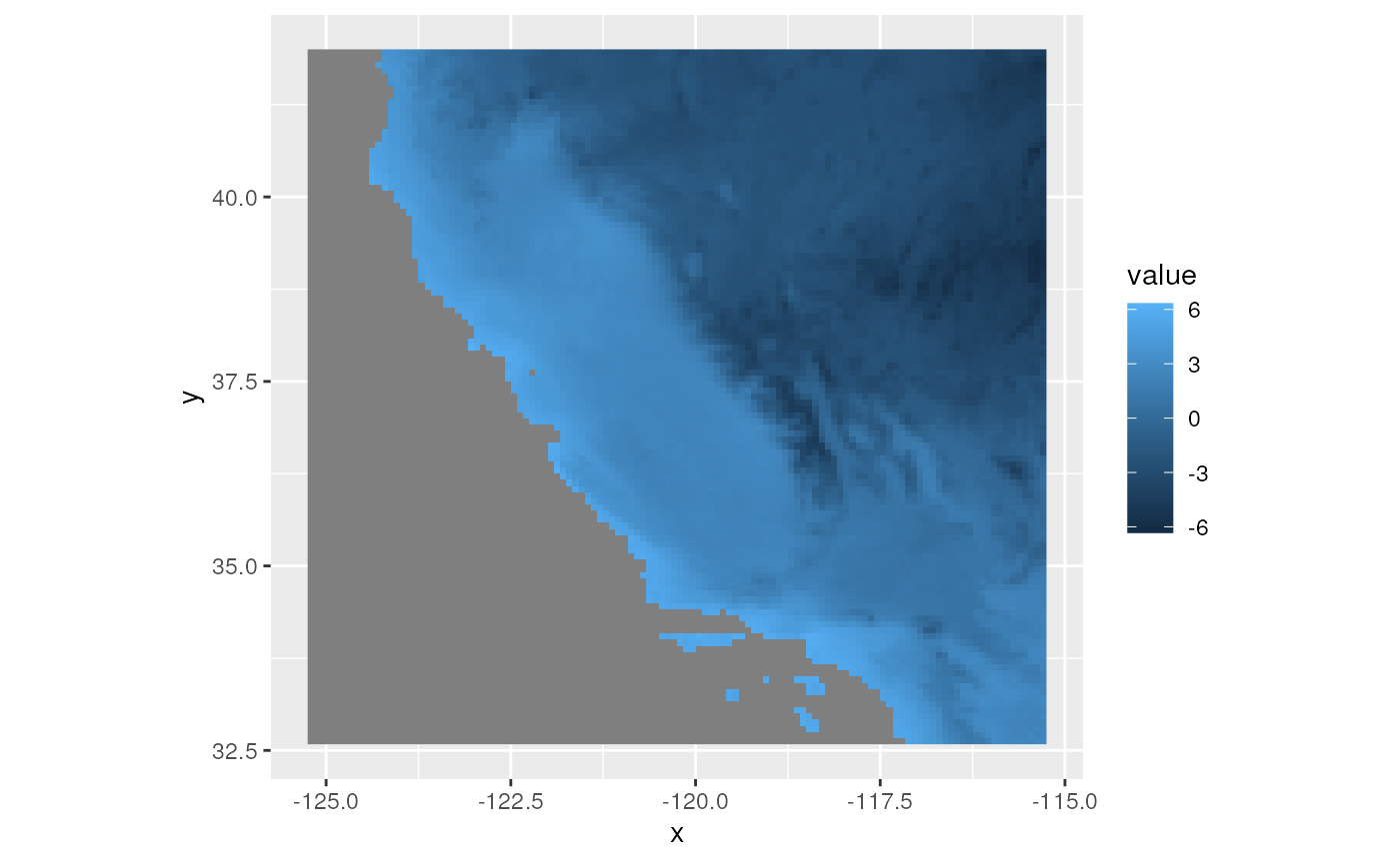
plots[[2]] 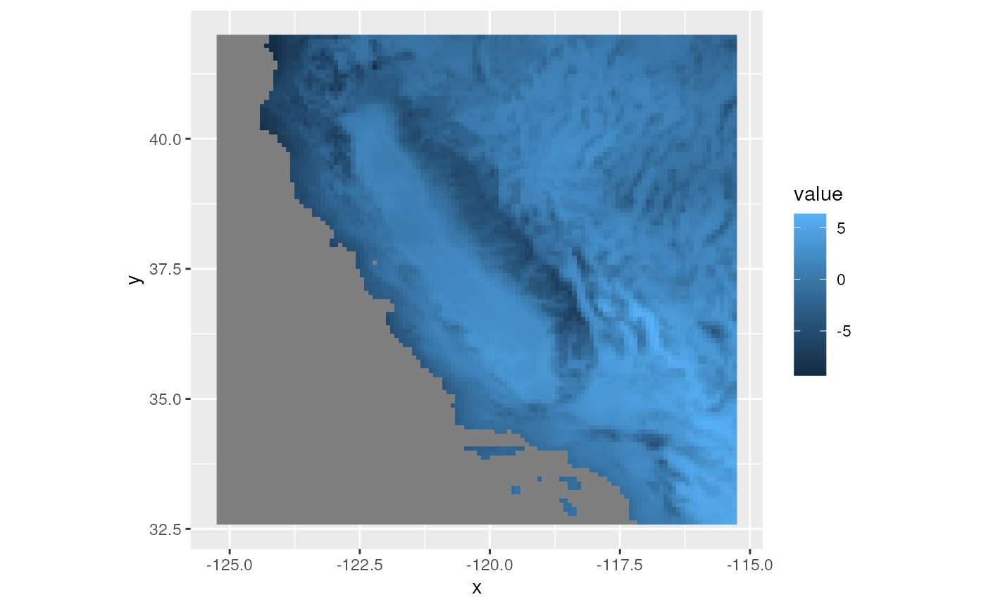
plots[[3]]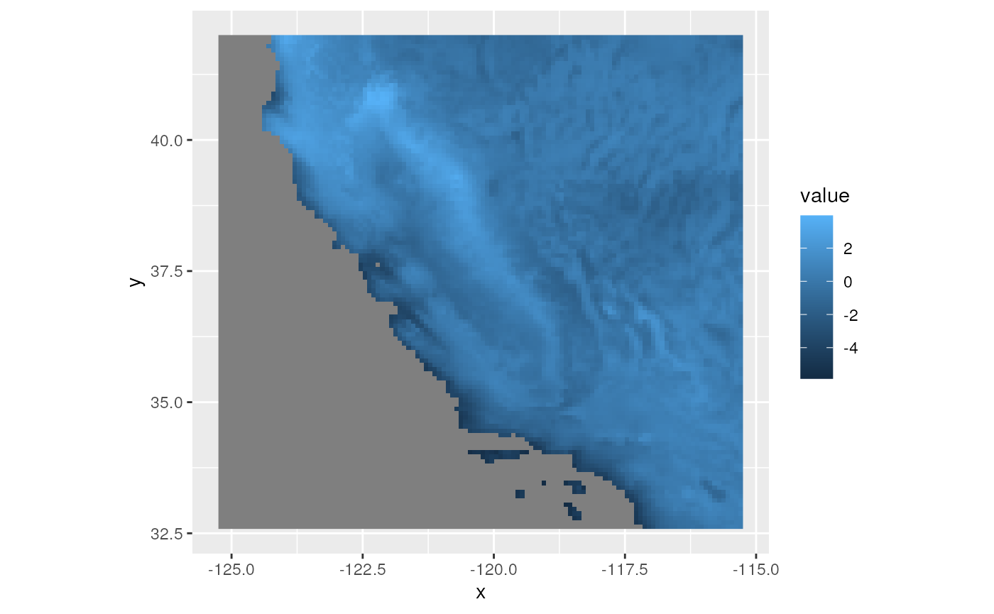
# We can also create a single composite raster plot with 3 PCs (each is assigned R, G, or B)
ggRGB(env_pcs$map, 1, 2, 3, stretch = "lin", q = 0, geom_raster = TRUE)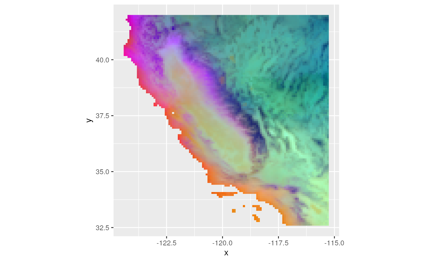
Create raster from coordinates with wingen:
coords_to_raster()
In some cases, we may not have a raster already prepared. Using the
wingen package, we can use our coordinate data to generate a raster
given a user-specified buffer around sampling coordinates (using the
buff argument) and with a given resolution (using the
res argument). This raster does not have any meaningful
values assigned to it, but can be used to create maps of genetic
diversity in wingen (see the wingen documentation here).
raster <- coords_to_raster(liz_coords, res = 1)
plot(raster, axes = FALSE)
points(liz_coords, pch = 19)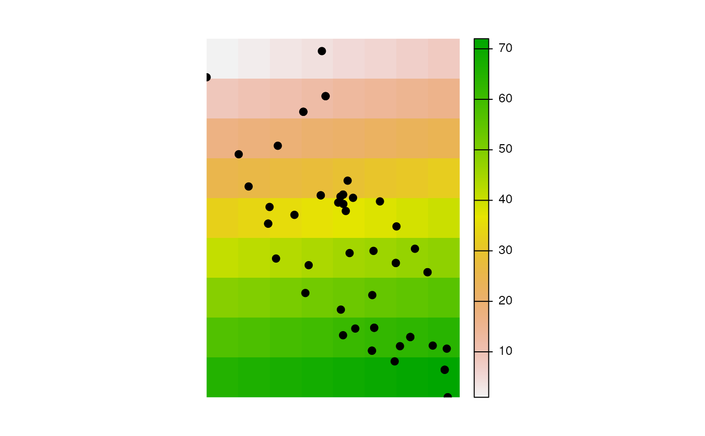
Calculate environmental distances using env_dist()
Some of the analyses within algatr, such as GDM and MMRR, require
comparing genetic distances to environmental distances. We can calculate
environmental distances using the env_dist() function,
which allows users to calculate environmental distances between
variables for given sampling locations. We first need to extract
environmental variables at sampling coordinates.
env <- raster::extract(CA_env, liz_coords)

# You can there are extracted values (n=53) for each environmental layer
head(env)
#>       CA_rPCA1   CA_rPCA2    CA_rPCA3
#> [1,] -1.851397 -3.9385712 -0.71366495
#> [2,] -2.288577 -0.7470118 -0.05549845
#> [3,] -4.294456  4.4240017 -1.50788176
#> [4,] -1.916433 -3.7858098 -1.37762737
#> [5,] -1.942174  0.2111327  1.20659840
#> [6,] -2.463599  4.4038172 -2.02557206
Now, we’re ready to calculate environmental distances.

We can make a heat map in ggplot with the pairwise distances.
as.data.frame(env_dist$CA_rPCA1) %>%
  rownames_to_column("sample") %>%
  pivot_longer(-"sample", names_to = "sample_comp", values_to = "dist") %>%
  ggplot(aes(x = as.numeric(sample), y = as.numeric(sample_comp), fill = dist)) +
  geom_tile() +
  coord_equal() +
  scale_fill_viridis() +
  xlab("Sample") +
  ylab("Sample")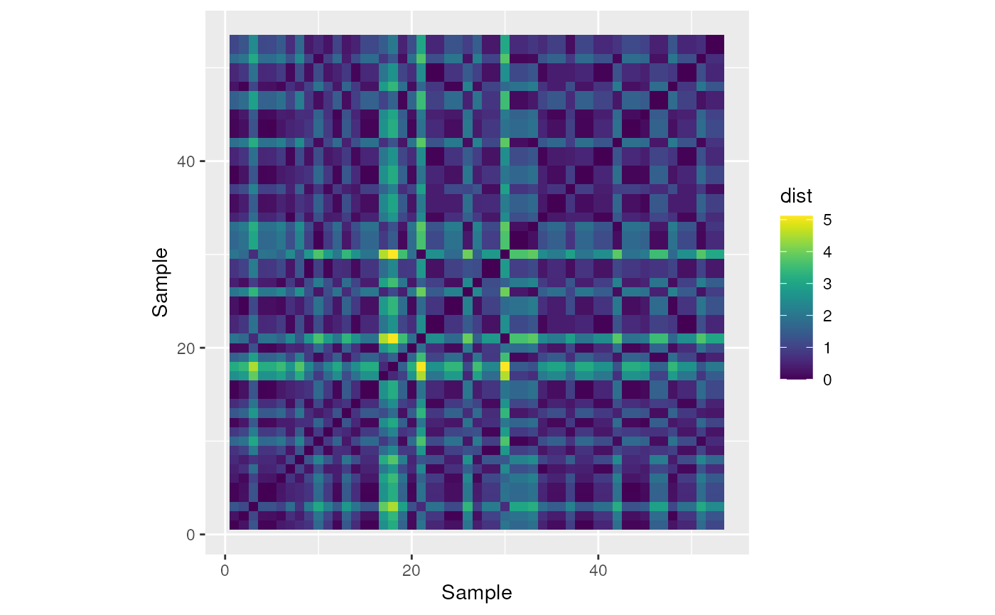
Calculate geographic distances using geo_dist()
The geo_dist() function allows users to choose from five
environmental distance metrics using the type argument:
Geodesic distances (
"euclidean"or"linear") using the geodist package (Padgham & Sumner 2021)Topographic distances (
"topo"or"topographic") using the topoDistance package (Wang 2020); requires a digital elevation model (DEM) raster specified with thelyrargumentResistance distances (
"resistance","cost", or"res") using the gdistance package (van Etten 2017); requires a resistance raster specified with thelyrargument
Euclidean distances

We can make a heat map in ggplot with the pairwise distances.
# Make a fun heat map with the pairwise distances
geo_dist <- as.data.frame(geo_dist)
colnames(geo_dist) <- rownames(geo_dist)
geo_dist %>%
  rownames_to_column("sample") %>%
  gather("sample_comp", "dist", -"sample") %>%
  ggplot(aes(x = as.numeric(sample), y = as.numeric(sample_comp), fill = dist)) +
  geom_tile() +
  coord_equal() +
  scale_fill_viridis() +
  xlab("Sample") +
  ylab("Sample")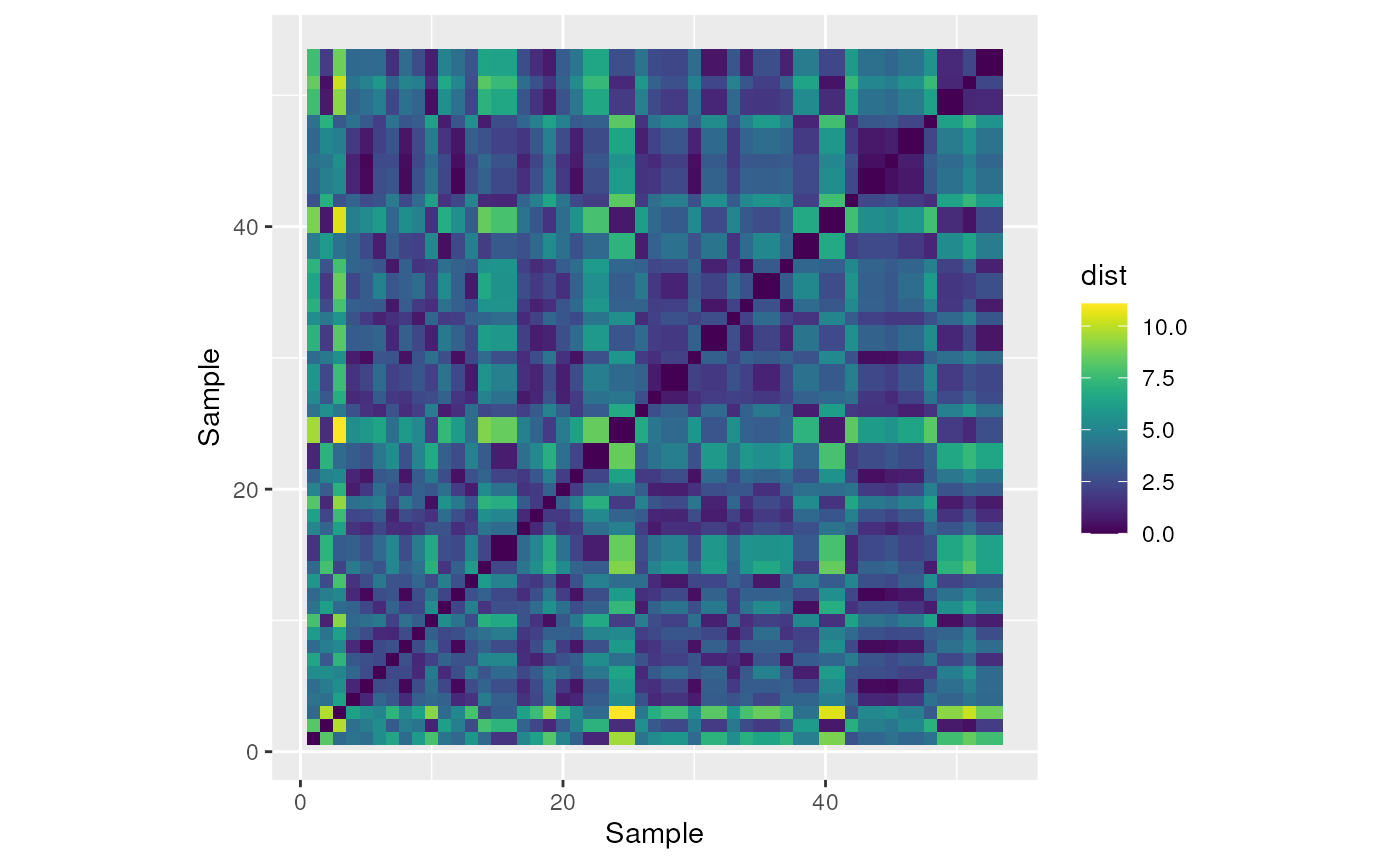
Topographic distances
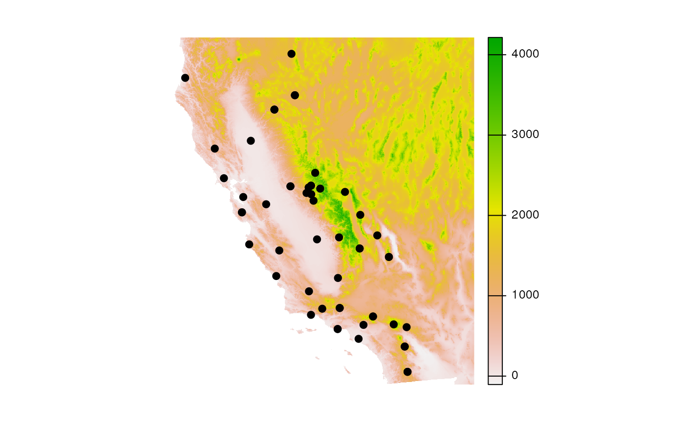
We can also calculate topographic distances, but need to provide a
digital elevation model (DEM) raster to do so. We can retrieve a DEM
using the geodata package, cropping to California using the
CA_env object in our example dataset.
# Download the DEM raster using the elevation_30s function
# This will save a .tif file in your current dir
dem <- elevation_30s(country = "USA", path = tempdir())
#> Cached as: /tmp/Rtmp6GYK9Q/elevation/USA_elv_msk.zip

# Crop to California limits
CA_dem <- crop(dem, CA_env)
Take a look at what the DEM looks like, with samples plotted on top.
Now, let’s calculate topographic distances using the
CA_dem object as our layer with the lyr
argument.
topo_dist <- geo_dist(liz_coords, type = "topo", lyr = CA_dem)
#> Calculating topo distances... This can be time consuming with many points and large rasters.
Plot the resulting topographic distances as a heatmap.
# Make a fun heat map with the pairwise distances
topo_dist <- as.data.frame(topo_dist)
colnames(topo_dist) <- 1:53
rownames(topo_dist) <- 1:53

topo_dist %>%
  rownames_to_column("sample") %>%
  gather("sample_comp", "dist", -"sample") %>%
  ggplot(aes(x = as.numeric(sample), y = as.numeric(sample_comp), fill = dist)) +
  geom_tile() +
  coord_equal() +
  scale_fill_viridis() +
  xlab("Sample") +
  ylab("Sample")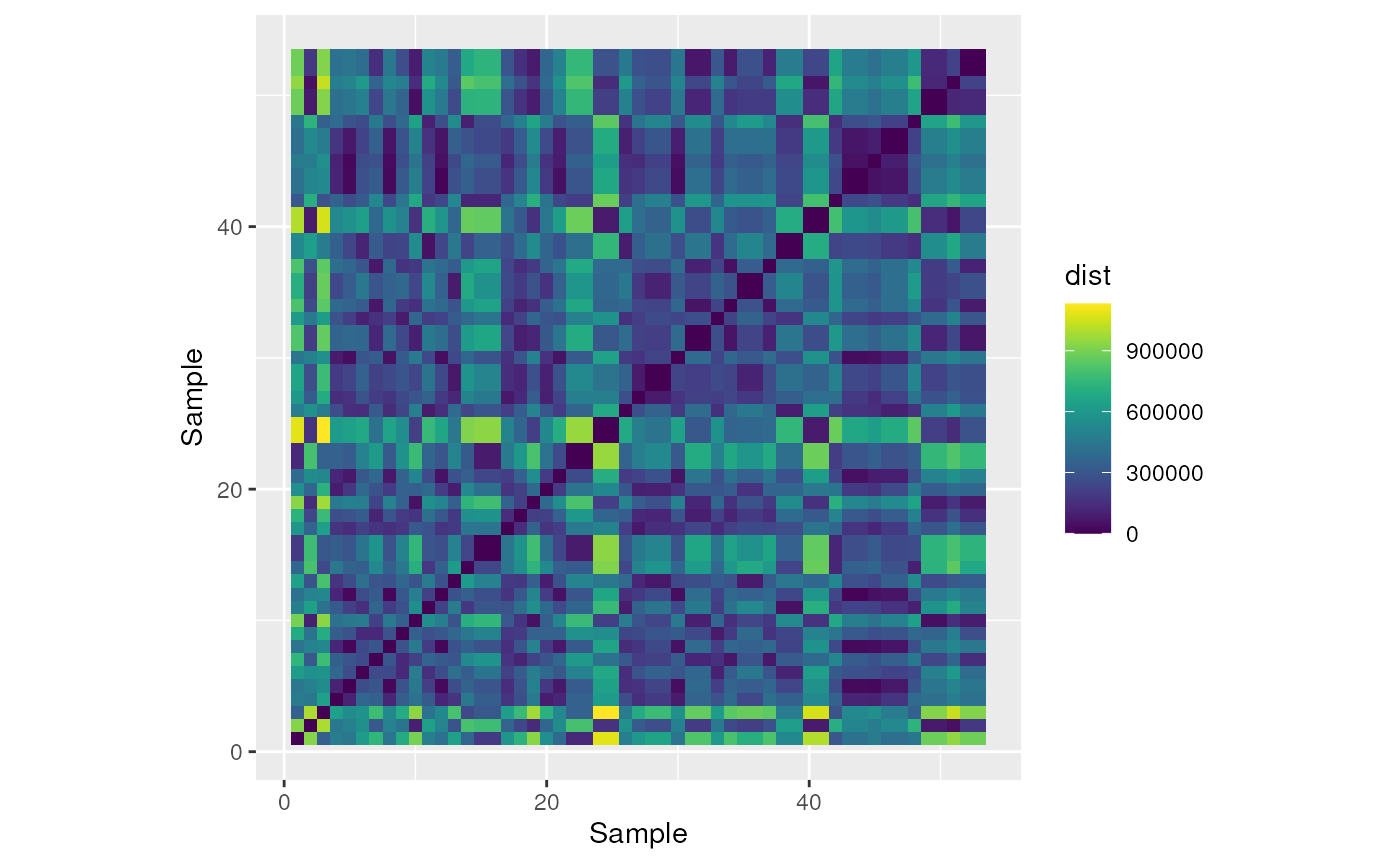
Additional documentation and citations
| Citation/URL | Details | |
|---|---|---|
| Associated code | terra (Hijmans 2022) and raster (Hijmans 2022) | algatr largely uses terra and raster packages to process and manipulate environmental data |
| Associated documentation | Walkthroughs for terra here and raster here | |
| Associated code | Padgham & Sumner 2021 | algatr uses the geodist package to calculate Euclidean distances |
| Associated code | Wang 2020 | algatr uses the topoDistance package to calculate topographic distances |
| Associated code | van Etten 2017; vignette available here | algatr uses the gdistance package to calculate resistance distances |
Retrieve relevant vignettes: