RDA
RDA_vignette.RmdRedundancy analysis (RDA)
#Install required packages
rda_packages()If using RDA, please cite the following: Capblancq T., Forester B.R. (2021) Redundancy analysis: A Swiss Army Knife for landscape genomics. Methods in Ecology and Evolution 12:2298-2309. DOI:10.1111/2041-210X.13722
Redundancy analysis (RDA) is a genotype-environment association (GEA) method that uses constrained ordination to detect outlier loci that are significantly associated with environmental variables. It does so by combining regression (in which response variables are genetic data, in our case, while explanatory variables are environmental data) with ordination (a PCA). Importantly, RDA is multivariate (i.e., multiple loci can be considered at a time), which is appealing in cases where multilocus selection may be occurring.
Model selection is performed by starting with a null model wherein the response is only explained by an intercept, and environmental variables are added until the amount of variance explained by a model that includes all variables is reached. By doing so, this method minimizes the redundancy among explanatory variables. Importantly, we can also perform an RDA that accounts for covariables (or “conditioning variables”) such as those that account for neutral population structure. When covariables are included, this is called a partial RDA. In algatr, population structure is quantified by running a PCA on the genetic data, and selecting a number of PC axes to best represent this type of neutral variation.
Some of the earliest examples of uses of RDA for identifying environment-associated loci are Lasky et al. 2012 and Forester et al. 2016. Since then, there have been several reviews and walkthroughs of the method that provide additional information, including workflows and comparisons with other GEA methods (e.g., Forester et al. 2018). Much of algatr’s code is adapted from one such paper, Capblancq & Forester 2021, the code of which is available here. algatr’s general workflow roughly follows the framework of Capblancq & Forester (2021).
RDA cannot take in missing values. Imputation based on the per-site
median is commonly performed, but there are several other ways
researchers can deal with missing values. For example, algatr contains
the str_impute() function to impute missing values based on
population structure using the LEA::impute() function.
However, here, we’ll opt to impute to the median, but strongly urge
researchers to use extreme caution when using this form of simplistic
imputation. We mainly provide code to impute on the median for testing
datasets and highly discourage its use in further analyses (please use
str_impute() instead!).
The general workflow to perform an RDA with algatr is as follows:
Simple vs. partial RDAs: We can run a simple RDA (no covariables) or partial RDA (conditioning covariables included) using
rda_run()Variable selection: Both simple and partial RDAs can be performed considering all variables (
"full"model) or by performing variable selection to determine variables that contribute most to genetic variance ("best"model)Variance partitioning: We can perform variance partitioning considering only variables that contribute significantly to genetic variance using
rda_varpart()Detecting outlier loci: Based on the results from above, we can detect outlier loci with
rda_getoutliers()
Read in and process genetic data
Running an RDA requires two data files for input: a genotype dosage
matrix (the gen argument) and the environmental values
extracted at sampling coordinates (the env argument). Let’s
first convert our vcf to a dosage matrix using the
vcf_to_dosage() function. N.B.: our code assumes that
sample IDs from our genetic data and our coords are in the same order;
be sure to check this before moving forward!
load_algatr_example()
#>
#> ---------------- example dataset ----------------
#>
#> Objects loaded:
#> *liz_vcf* vcfR object (1000 loci x 53 samples)
#> *liz_gendist* genetic distance matrix (Plink Distance)
#> *liz_coords* dataframe with x and y coordinates
#> *CA_env* RasterStack with example environmental layers
#>
#> -------------------------------------------------
#>
#>
# Convert from vcf to dosage matrix:
gen <- vcf_to_dosage(liz_vcf)
#> Loading required namespace: vcfR
#> Loading required namespace: adegenet
As mentioned above, running an RDA requires that your genotype matrix contains no missing values. Let’s impute missing values based on the per-site median. N.B.: this type of simplistic imputation is strongly not recommended for downstream analyses and is used here for example’s sake!
# Are there NAs in the data?
gen[1:5, 1:5]
#>        Locus_10 Locus_15 Locus_22 Locus_28 Locus_32
#> ALT3          0        0        0        0        0
#> BAR360        0        0        0       NA        0
#> BLL5          0       NA        0        0       NA
#> BNT5          0        0       NA       NA        0
#> BOF1          0       NA       NA       NA       NA
gen <- simple_impute(gen)
# Check that NAs are gone
gen[1:5, 1:5]
#>        Locus_10 Locus_15 Locus_22 Locus_28 Locus_32
#> ALT3          0        0        0        0        0
#> BAR360        0        0        0        0        0
#> BLL5          0        0        0        0        0
#> BNT5          0        0        0        0        0
#> BOF1          0        0        0        0        0
Process environmental data
Let’s extract environmental variables using the
extract() function from the raster package. We also need to
standardize environmental variables. This is particularly important if
we are using (for example) bioclimatic variables as input, as units of
measurement are completely different (e.g., mm for precipitation
vs. degrees Celsius for temperature). To do so, we’ll use the
scale() function within the raster package.
# Extract environmental vars
env <- raster::extract(CA_env, liz_coords)

# Standardize environmental variables and make into dataframe
env <- scale(env, center = TRUE, scale = TRUE)
env <- data.frame(env)
Running simple and partial RDAs using rda_run(), with
and without variable selection
The main function within algatr to perform an RDA is
rda_run(), which uses the rda() function
within the vegan package.
Run a simple RDA with no variable selection
A simple RDA is one in which our model will not account for
covariables in the model, and is the default for rda_run().
Let’s first run a simple RDA on all environmental variables (i.e., no
variable selection). This is specified using the
model = "full" argument.
mod_full <- rda_run(gen, env, model = "full")The resulting object is large, containing 12 elements relevant to the RDA. Let’s take a look at what function was called. We can see that all environmental variables (CA_rPCA1, 2, and 3) were included in the model, and that geography or structure were not included in the model (and there were no conditioning variables).
mod_full$call
#> rda(formula = gen ~ CA_rPCA1 + CA_rPCA2 + CA_rPCA3, data = moddf)
Now, let’s take a look at the summary of this model. One of the most important parts of this object is the partitioning of variance. Within an RDA, the term “inertia” can be interpreted as variance, and our results show us that the amount of variance explained by explanatory variables alone (constrained inertia) is only 9.768%. Unconstrained inertia is the residual variance, which is very high (90.232%). The summary also provides site scores, site constraints, and biplot scores.
summary(mod_full)
#>
#> Call:
#> rda(formula = gen ~ CA_rPCA1 + CA_rPCA2 + CA_rPCA3, data = moddf)
#>
#> Partitioning of variance:
#>               Inertia Proportion
#> Total          143.39    1.00000
#> Constrained     14.01    0.09768
#> Unconstrained  129.38    0.90232
#>
#> Eigenvalues, and their contribution to the variance
#>
#> Importance of components:
#>                          RDA1    RDA2    RDA3     PC1     PC2     PC3     PC4
#> Eigenvalue            7.28806 4.98205 1.73568 18.6608 9.31326 7.51572 5.53312
#> Proportion Explained  0.05083 0.03474 0.01210  0.1301 0.06495 0.05241 0.03859
#> Cumulative Proportion 0.05083 0.08557 0.09768  0.2278 0.29277 0.34518 0.38377
#>                           PC5    PC6     PC7     PC8     PC9    PC10    PC11
#> Eigenvalue            4.51893 4.0443 3.69111 3.30413 3.09940 3.04539 3.00412
#> Proportion Explained  0.03152 0.0282 0.02574 0.02304 0.02162 0.02124 0.02095
#> Cumulative Proportion 0.41529 0.4435 0.46923 0.49228 0.51389 0.53513 0.55608
#>                          PC12    PC13    PC14    PC15    PC16   PC17    PC18
#> Eigenvalue            2.83164 2.80969 2.74342 2.58682 2.47393 2.4664 2.32471
#> Proportion Explained  0.01975 0.01959 0.01913 0.01804 0.01725 0.0172 0.01621
#> Cumulative Proportion 0.57583 0.59542 0.61456 0.63260 0.64985 0.6671 0.68326
#>                          PC19    PC20    PC21    PC22    PC23    PC24    PC25
#> Eigenvalue            2.29159 2.22955 2.15249 2.10481 2.01172 1.94388 1.90538
#> Proportion Explained  0.01598 0.01555 0.01501 0.01468 0.01403 0.01356 0.01329
#> Cumulative Proportion 0.69925 0.71480 0.72981 0.74449 0.75852 0.77207 0.78536
#>                          PC26    PC27    PC28    PC29    PC30    PC31    PC32
#> Eigenvalue            1.82439 1.79687 1.68505 1.64293 1.59963 1.56602 1.50690
#> Proportion Explained  0.01272 0.01253 0.01175 0.01146 0.01116 0.01092 0.01051
#> Cumulative Proportion 0.79808 0.81062 0.82237 0.83382 0.84498 0.85590 0.86641
#>                          PC33     PC34    PC35     PC36    PC37     PC38
#> Eigenvalue            1.46174 1.433419 1.34638 1.331355 1.28477 1.253763
#> Proportion Explained  0.01019 0.009997 0.00939 0.009285 0.00896 0.008744
#> Cumulative Proportion 0.87661 0.886602 0.89599 0.905277 0.91424 0.922981
#>                          PC39     PC40    PC41     PC42     PC43     PC44
#> Eigenvalue            1.23738 1.175289 1.13416 1.072082 1.067608 1.017457
#> Proportion Explained  0.00863 0.008197 0.00791 0.007477 0.007446 0.007096
#> Cumulative Proportion 0.93161 0.939807 0.94772 0.955193 0.962639 0.969734
#>                           PC45     PC46     PC47     PC48     PC49
#> Eigenvalue            0.998927 0.910062 0.866439 0.836444 0.727872
#> Proportion Explained  0.006967 0.006347 0.006043 0.005833 0.005076
#> Cumulative Proportion 0.976701 0.983048 0.989090 0.994924 1.000000
#>
#> Accumulated constrained eigenvalues
#> Importance of components:
#>                         RDA1   RDA2   RDA3
#> Eigenvalue            7.2881 4.9820 1.7357
#> Proportion Explained  0.5204 0.3557 0.1239
#> Cumulative Proportion 0.5204 0.8761 1.0000
One of the most relevant statistics to present from an RDA model is the adjusted R2 value. The R2 value must be adjusted; if not, it is biased because it will always increase if independent variables are added (i.e., there is no penalization for adding independent variables that aren’t significantly affecting dependent variables within the model). The adjusted R2 value from the full (global) model can also help us determine the stopping point when we go on to do variable selection. As we can see, the unadjusted R2 is 0.098, while the adjusted value is 0.042. Be sure to always report adjusted R2 values.
RsquareAdj(mod_full)
#> $r.squared
#> [1] 0.0976769
#>
#> $adj.r.squared
#> [1] 0.04243263
Run a simple RDA with variable selection
Now, let’s run an RDA model with variable selection by specifying the
"best" model within rda_run(). Variable
selection occurs using the ordiR2step() function in the
vegan package, and is a forward selection method that begins with a null
model and adds explanatory variables one at a time until genetic
variance is maximized. To perform forward selection, we need to specify
stopping criteria (i.e., when to stop adding more explanatory
variables). There are two primary ways to specify stopping criteria:
parameters involved in a permutation-based significance test (two
parameters: the limits of permutation p-values for adding
(Pin) or dropping (Pout) a term to the model,
and the number of permutations used in the estimation of adjusted R2
(R2permutations)), and whether to use the adjusted R2 value
as the stopping criterion (R2scope; only models with
adjusted R2 values lower than specified are accepted).
mod_best <- rda_run(gen, env,
  model = "best",
  Pin = 0.05,
  R2permutations = 1000,
  R2scope = T
)
#> Step: R2.adj= 0
#> Call: gen ~ 1
#>
#>                  R2.adjusted
#> <All variables> 0.0424326339
#> + CA_rPCA2      0.0196214014
#> + CA_rPCA3      0.0137427906
#> + CA_rPCA1      0.0009953656
#> <model>         0.0000000000
#>
#>            Df    AIC      F Pr(>F)
#> + CA_rPCA2  1 264.09 2.0407  0.002 **
#> ---
#> Signif. codes:  0 '***' 0.001 '**' 0.01 '*' 0.05 '.' 0.1 ' ' 1
#>
#> Step: R2.adj= 0.0196214
#> Call: gen ~ CA_rPCA2
#>
#>                 R2.adjusted
#> <All variables>  0.04243263
#> + CA_rPCA3       0.03919420
#> + CA_rPCA1       0.01991617
#> <model>          0.01962140
#>
#>            Df    AIC      F Pr(>F)
#> + CA_rPCA3  1 263.97 2.0389  0.006 **
#> ---
#> Signif. codes:  0 '***' 0.001 '**' 0.01 '*' 0.05 '.' 0.1 ' ' 1
#>
#> Step: R2.adj= 0.0391942
#> Call: gen ~ CA_rPCA2 + CA_rPCA3
#>
#>                 R2.adjusted
#> <All variables>  0.04243263
#> + CA_rPCA1       0.04243263
#> <model>          0.03919420
#>
#>            Df    AIC      F Pr(>F)
#> + CA_rPCA1  1 264.72 1.1691   0.17
Let’s look at our best model, and see how it compares to our full
model. There is also an additional element in the mod_best
object, which are the results from an ANOVA-like permutation test. When
we look at the call, we can now see that only environmental PCs 2 and 3
are considered in the model, meaning that PC1 is not considered to be
significantly associated with genetic variance. Importantly, our
adjusted R2 value is 0.039 (compared to 0.042 for the full model), which
tells us that the model with only two of the environmental variables
explains nearly as much as the RDA with all three.
mod_best$call
#> rda(formula = gen ~ CA_rPCA2 + CA_rPCA3, data = list(CA_rPCA1 = c(-0.522839974379508,
#> -0.762922496792446, -1.86447664460538, -0.55855495052221, -0.57269132662902,
#> -0.859038227685075, -0.072043636015037, -1.13434251082331, 0.213097754647621,
#> 1.17658258339642, 0.297967827057378, -0.464084951296452, 0.855636561890484,
#> 0.0953591037247294, -0.539120600258253, -0.539120600258253, 2.02106276091047,
#> 2.60771978346453, 1.05200372725675, -0.629034085084968, -2.46854442016198,
#> 0.0260725501626235, 0.0260725501626235, -0.746727041242616, -0.746727041242616,
#> 1.47817418774494, -0.936256358142168, 0.237069667112143, 0.237069667112143,
#> -2.50772800868535, 1.1549776008528, 1.1549776008528, 1.35110535969113,
#> -0.0561341328070219, -0.373693242601386, -0.373693242601386,
#> 0.399649342383328, -0.519583011248178, -0.519583011248178, -0.00782108370036044,
#> -0.00782108370036044, 1.31832335901042, -0.576916652177962, -0.576916652177962,
#> -0.431388317340501, 1.01567982581473, 1.01567982581473, -0.774971381524837,
#> 0.0255686311719819, 0.0255686311719819, 1.23221556728965, 0.562570108128171,
#> 0.562570108128171), CA_rPCA2 = c(-1.73421968589969, -0.495566879281243,
#> 1.51131736830612, -1.67493255235748, -0.123708413803996, 1.50348370296656,
#> 0.497816234346518, -0.0361828529216023, 1.45881385953799, 1.05507640816238,
#> 1.16578925063956, -0.171884322138841, -1.48147701298751, 0.73732782244215,
#> -0.24074966665597, -0.24074966665597, 0.0399288951693412, -0.0168067684167015,
#> 1.50893728869516, -1.66080206726807, -1.26905097514619, -1.58120699373763,
#> -1.58120699373763, -0.318166617922595, -0.318166617922595, 0.180021614507387,
#> -0.0989825979307121, -0.816171384725929, -0.816171384725929,
#> -1.07421654041962, 0.421584519953747, 0.421584519953747, 0.118248661677072,
#> 0.574145244972511, -1.3512331198936, -1.3512331198936, 1.75926629328248,
#> 1.0258059259489, 1.0258059259489, -0.436435405832552, -0.436435405832552,
#> 0.225239240818199, -0.306788498922838, -0.306788498922838, -0.0148935881217706,
#> 0.167555482577237, 0.167555482577237, 1.53563948346279, -0.0452634761317479,
#> -0.0452634761317479, -0.608661189332775, 1.77623627386297, 1.77623627386297
#> ), CA_rPCA3 = c(-0.171546498077063, 0.304720882227611, -0.746263624095161,
#> -0.652007967024141, 1.21800886957269, -1.12087856243146, -0.0660703381728475,
#> 1.19845138122507, -2.64925798891154, 0.00947773794228616, -1.44942908084647,
#> 1.08487356159833, -0.149185156402174, 1.50244347942537, 2.13591256195157,
#> 2.13591256195157, 0.263989245701077, 0.527413437472692, -1.87246014428684,
#> -0.874873913836537, -0.467712504092297, 0.0665799769739865, 0.0665799769739865,
#> 0.0384364183523902, 0.0384364183523902, 0.0320667279913713, -0.0354734132813299,
#> -0.233862027212001, -0.233862027212001, -0.817475641342106, -0.0125888642166748,
#> -0.0125888642166748, 0.0520076559082537, -0.559760860443754,
#> -0.540788236051066, -0.540788236051066, -1.79928400205617, -0.331431611440013,
#> -0.331431611440013, 0.230740506231628, 0.230740506231628, 0.709448526300272,
#> 0.943896504682603, 0.943896504682603, 1.33634384148885, 1.23383642686616,
#> 1.23383642686616, 0.0143927948732277, 0.714359011285843, 0.714359011285843,
#> 0.339745387114261, -1.82594258419516, -1.82594258419516)))
mod_best$anova
#>                   R2.adj Df    AIC      F Pr(>F)
#> + CA_rPCA2      0.019621  1 264.09 2.0407  0.002 **
#> + CA_rPCA3      0.039194  1 263.97 2.0389  0.006 **
#> <All variables> 0.042433
#> ---
#> Signif. codes:  0 '***' 0.001 '**' 0.01 '*' 0.05 '.' 0.1 ' ' 1
RsquareAdj(mod_best)
#> $r.squared
#> [1] 0.07614827
#>
#> $adj.r.squared
#> [1] 0.0391942
Following variable selection, we want to retain two environmental variables (CA_rPCA2 and CA_rPCA3) for all subsequent analyses.
Run a partial RDA with geography as a covariable
A partial RDA, as described at the beginning of the vignette, is when
covariables (or conditioning variables) are incorporated into the RDA.
Within rda_run(), to correct for geography, users can set
correctGEO = TRUE, in which case sampling coordinates
(coords) must also be provided. Let’s now run a partial
RDA, without any variable selection (the full model) and view the
results.
mod_pRDA_geo <- rda_run(gen, env, liz_coords,
  model = "full",
  correctGEO = TRUE,
  correctPC = FALSE
)
Let’s take a look at our partial RDA results. Note that now, the call
includes conditioning variables x and y, which correspond to our
latitude and longitude values. Conditioning variables are specified
within the rda() function using the
Condition() function. Finally, when we look at the summary
of the resulting object, we can see that along with total, constrained,
and unconstrained inertia (or variance) as with our simple RDA, there is
an additional row for conditioned inertia because our partial RDA
includes conditioning variables. Interestingly, the conditioned inertia
is higher than constrained inertia, suggesting that geography is more
associated with genetic variance than our environmental variables
are.
anova(mod_pRDA_geo)
#> Permutation test for rda under reduced model
#> Permutation: free
#> Number of permutations: 999
#>
#> Model: rda(formula = gen ~ CA_rPCA1 + CA_rPCA2 + CA_rPCA3 + Condition(x + y), data = moddf)
#>          Df Variance      F Pr(>F)
#> Model     3   11.306 1.5948  0.001 ***
#> Residual 47  111.068
#> ---
#> Signif. codes:  0 '***' 0.001 '**' 0.01 '*' 0.05 '.' 0.1 ' ' 1
RsquareAdj(mod_pRDA_geo) # 0.0305
#> $r.squared
#> [1] 0.07884828
#>
#> $adj.r.squared
#> [1] 0.03058243
summary(mod_pRDA_geo)
#>
#> Call:
#> rda(formula = gen ~ CA_rPCA1 + CA_rPCA2 + CA_rPCA3 + Condition(x +      y), data = moddf)
#>
#> Partitioning of variance:
#>               Inertia Proportion
#> Total          143.39    1.00000
#> Conditioned     21.01    0.14656
#> Constrained     11.31    0.07885
#> Unconstrained  111.07    0.77459
#>
#> Eigenvalues, and their contribution to the variance
#> after removing the contribution of conditiniong variables
#>
#> Importance of components:
#>                          RDA1    RDA2    RDA3      PC1     PC2     PC3     PC4
#> Eigenvalue            6.87372 2.80216 1.63009 11.00385 7.49907 5.16346 4.68171
#> Proportion Explained  0.05617 0.02290 0.01332  0.08992 0.06128 0.04219 0.03826
#> Cumulative Proportion 0.05617 0.07907 0.09239  0.18231 0.24359 0.28578 0.32404
#>                           PC5     PC6     PC7     PC8     PC9    PC10    PC11
#> Eigenvalue            4.21148 3.72312 3.45801 3.19495 3.01860 2.98188 2.93280
#> Proportion Explained  0.03441 0.03042 0.02826 0.02611 0.02467 0.02437 0.02397
#> Cumulative Proportion 0.35845 0.38888 0.41714 0.44324 0.46791 0.49228 0.51624
#>                          PC12    PC13   PC14    PC15    PC16    PC17    PC18
#> Eigenvalue            2.79673 2.59175 2.5826 2.49887 2.45425 2.32321 2.29777
#> Proportion Explained  0.02285 0.02118 0.0211 0.02042 0.02006 0.01898 0.01878
#> Cumulative Proportion 0.53910 0.56028 0.5814 0.60180 0.62186 0.64084 0.65962
#>                          PC19    PC20    PC21    PC22    PC23   PC24    PC25
#> Eigenvalue            2.15916 2.14664 2.03834 2.00771 1.91618 1.8479 1.80441
#> Proportion Explained  0.01764 0.01754 0.01666 0.01641 0.01566 0.0151 0.01475
#> Cumulative Proportion 0.67726 0.69480 0.71146 0.72787 0.74352 0.7586 0.77337
#>                         PC26    PC27    PC28    PC29    PC30    PC31    PC32
#> Eigenvalue            1.7740 1.68265 1.64600 1.58626 1.52630 1.47782 1.45805
#> Proportion Explained  0.0145 0.01375 0.01345 0.01296 0.01247 0.01208 0.01191
#> Cumulative Proportion 0.7879 0.80162 0.81507 0.82803 0.84050 0.85258 0.86449
#>                          PC33    PC34    PC35    PC36    PC37     PC38     PC39
#> Eigenvalue            1.42866 1.37519 1.30318 1.27465 1.24443 1.221578 1.169694
#> Proportion Explained  0.01167 0.01124 0.01065 0.01042 0.01017 0.009982 0.009558
#> Cumulative Proportion 0.87617 0.88741 0.89805 0.90847 0.91864 0.928622 0.938181
#>                           PC40     PC41     PC42     PC43     PC44     PC45
#> Eigenvalue            1.073702 1.068009 1.045150 1.006285 0.935246 0.866846
#> Proportion Explained  0.008774 0.008727 0.008541 0.008223 0.007643 0.007084
#> Cumulative Proportion 0.946955 0.955682 0.964223 0.972446 0.980088 0.987172
#>                           PC46     PC47
#> Eigenvalue            0.841414 0.728431
#> Proportion Explained  0.006876 0.005952
#> Cumulative Proportion 0.994048 1.000000
#>
#> Accumulated constrained eigenvalues
#> Importance of components:
#>                        RDA1   RDA2   RDA3
#> Eigenvalue            6.874 2.8022 1.6301
#> Proportion Explained  0.608 0.2478 0.1442
#> Cumulative Proportion 0.608 0.8558 1.0000
Run a partial RDA with population genetic structure and geography as covariables
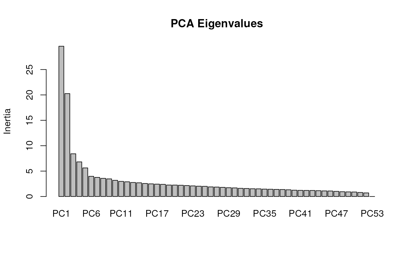
Lastly, let’s run a partial RDA with both geography
(correctGEO = TRUE) and population structure
(correctPC = TRUE) as conditioning variables. Within
algatr, population structure is quantified using a PCA, and a user can
specify the number of axes to retain in the RDA model. In this case,
we’ll retain three axes, which we can specify using the nPC
argument. If this argument is set to "manual", a screeplot
will be printed and a user can manually enter the number of PCs that
they feel best describe the data.
mod_pRDA_gs <- rda_run(gen, env, liz_coords,
  model = "full",
  correctGEO = TRUE,
  correctPC = TRUE,
  nPC = 3
)
Now, we see that even more inertia/variance is explained by the conditioning variables.
summary(mod_pRDA_gs)
#>
#> Call:
#> rda(formula = gen ~ CA_rPCA1 + CA_rPCA2 + CA_rPCA3 + Condition(PC1 +      PC2 + PC3 + x + y), data = moddf)
#>
#> Partitioning of variance:
#>               Inertia Proportion
#> Total         143.389    1.00000
#> Conditioned    48.063    0.33519
#> Constrained     6.672    0.04653
#> Unconstrained  88.654    0.61828
#>
#> Eigenvalues, and their contribution to the variance
#> after removing the contribution of conditiniong variables
#>
#> Importance of components:
#>                          RDA1    RDA2    RDA3     PC1     PC2     PC3     PC4
#> Eigenvalue            2.72234 2.30006 1.64942 5.15035 4.44551 3.82383 3.55107
#> Proportion Explained  0.02856 0.02413 0.01730 0.05403 0.04663 0.04011 0.03725
#> Cumulative Proportion 0.02856 0.05269 0.06999 0.12402 0.17065 0.21077 0.24802
#>                           PC5     PC6     PC7     PC8     PC9    PC10    PC11
#> Eigenvalue            3.24764 3.02810 2.99645 2.95013 2.79913 2.65085 2.59129
#> Proportion Explained  0.03407 0.03177 0.03143 0.03095 0.02936 0.02781 0.02718
#> Cumulative Proportion 0.28209 0.31385 0.34529 0.37623 0.40560 0.43341 0.46059
#>                          PC12    PC13    PC14    PC15    PC16    PC17    PC18
#> Eigenvalue            2.52112 2.46520 2.34331 2.30029 2.16258 2.15304 2.05042
#> Proportion Explained  0.02645 0.02586 0.02458 0.02413 0.02269 0.02259 0.02151
#> Cumulative Proportion 0.48704 0.51290 0.53748 0.56161 0.58430 0.60688 0.62839
#>                          PC19    PC20    PC21   PC22    PC23    PC24    PC25
#> Eigenvalue            2.01366 1.92134 1.85435 1.8112 1.79300 1.68266 1.65184
#> Proportion Explained  0.02112 0.02016 0.01945 0.0190 0.01881 0.01765 0.01733
#> Cumulative Proportion 0.64952 0.66967 0.68912 0.7081 0.72693 0.74458 0.76191
#>                          PC26    PC27    PC28    PC29    PC30    PC31    PC32
#> Eigenvalue            1.58977 1.52980 1.47897 1.46048 1.44680 1.38037 1.30440
#> Proportion Explained  0.01668 0.01605 0.01551 0.01532 0.01518 0.01448 0.01368
#> Cumulative Proportion 0.77859 0.79464 0.81015 0.82547 0.84065 0.85513 0.86882
#>                          PC33    PC34    PC35    PC36    PC37    PC38    PC39
#> Eigenvalue            1.27639 1.24668 1.22365 1.17070 1.07515 1.06819 1.05602
#> Proportion Explained  0.01339 0.01308 0.01284 0.01228 0.01128 0.01121 0.01108
#> Cumulative Proportion 0.88221 0.89528 0.90812 0.92040 0.93168 0.94289 0.95396
#>                          PC40     PC41    PC42     PC43     PC44
#> Eigenvalue            1.00764 0.940164 0.86839 0.842461 0.729857
#> Proportion Explained  0.01057 0.009863 0.00911 0.008838 0.007656
#> Cumulative Proportion 0.96453 0.974396 0.98351 0.992344 1.000000
#>
#> Accumulated constrained eigenvalues
#> Importance of components:
#>                        RDA1   RDA2   RDA3
#> Eigenvalue            2.722 2.3001 1.6494
#> Proportion Explained  0.408 0.3447 0.2472
#> Cumulative Proportion 0.408 0.7528 1.0000
Variance partitioning with partial RDA
In many cases, we want to understand the independent contributions of each explanatory variable in combination with our covariables. Also, we can understand how much confounded variance there is (i.e., variation that is explained by the combination of multiple explanatory variables). The best way to do this is to run partial RDAs on each set of explanatory variables and examine the inertia of each pRDA result as it compares to the full model. In this case, the full model is an RDA that considers neutral processes as explanatory variables rather than conditioning variables (covariables).
The call for this full model looks like this:
rda(gen ~ env + covariable, data), rather than a true
partial RDA which would take the form:
rda(gen ~ env + Condition(covariable), data).
In algatr, we can run variance partitioning using the function
rda_varpart(), which will run the full model (as above) and
then will run successive pRDAs which are conditioned on three successive
sets of variables. These variable sets are significant environmental
variables (in our case, environmental PCs 2 and 3), population genetic
structure (once again determined using a PC with a user-specified number
of PC axes), and geography (sampling coordinates). This function will
then provide us with information on how variance is partitioned in the
form of a table containing relevant statistics; this table is nearly
identical to Table 2 from Capblancq
& Forester 2021. The rda_varpart() parameters are
identical to those from rda_run(). As with
rda_run(), we can provide a number for the number of PCs to
consider for population structure (nPC), or this argument
can be set to "manual" if a user would like to manually
enter a number into the console after viewing the screeplot. We can then
use rda_varpart_table() to visualize these results in an
aesthetically pleasing way; users can specify whether to display the
function call in the table (call_col; defaults to
FALSE) and the number of digits to round to
digits (the default is 2).
varpart <- rda_varpart(gen, env, liz_coords,
  Pin = 0.05, R2permutations = 1000,
  R2scope = T, nPC = 3
)
#> Step: R2.adj= 0
#> Call: gen ~ 1
#>
#>                  R2.adjusted
#> <All variables> 0.0424326339
#> + CA_rPCA2      0.0196214014
#> + CA_rPCA3      0.0137427906
#> + CA_rPCA1      0.0009953656
#> <model>         0.0000000000
#>
#>            Df    AIC      F Pr(>F)
#> + CA_rPCA2  1 264.09 2.0407  0.004 **
#> ---
#> Signif. codes:  0 '***' 0.001 '**' 0.01 '*' 0.05 '.' 0.1 ' ' 1
#>
#> Step: R2.adj= 0.0196214
#> Call: gen ~ CA_rPCA2
#>
#>                 R2.adjusted
#> <All variables>  0.04243263
#> + CA_rPCA3       0.03919420
#> + CA_rPCA1       0.01991617
#> <model>          0.01962140
#>
#>            Df    AIC      F Pr(>F)
#> + CA_rPCA3  1 263.97 2.0389  0.006 **
#> ---
#> Signif. codes:  0 '***' 0.001 '**' 0.01 '*' 0.05 '.' 0.1 ' ' 1
#>
#> Step: R2.adj= 0.0391942
#> Call: gen ~ CA_rPCA2 + CA_rPCA3
#>
#>                 R2.adjusted
#> <All variables>  0.04243263
#> + CA_rPCA1       0.04243263
#> <model>          0.03919420
#>
#>            Df    AIC      F Pr(>F)
#> + CA_rPCA1  1 264.72 1.1691  0.164
rda_varpart_table(varpart, call_col = TRUE)| Variance partitioning | |||||||
| Model | pRDA model call | Inertia | R2 | Adjusted R2 | p (>F) | Prop. of explainable variance | Prop. of total variance |
|---|---|---|---|---|---|---|---|
| Full model | gen ~ CA_rPCA2 + CA_rPCA3 + PC1 + PC2 + PC3 + x + y | 52.67 | 0.37 | 0.27 | 0.00 | 1.00 | 0.37 |
| Pure enviro. model | gen ~ CA_rPCA2 + CA_rPCA3 + Condition(PC1 + PC2 + PC3 + x + y) | 4.61 | 0.03 | 0.00 | 0.03 | 0.09 | 0.03 |
| Pure pop. structure model | gen ~ PC1 + PC2 + PC3 + Condition(CA_rPCA2 + CA_rPCA3 + x + y) | 23.09 | 0.16 | 0.13 | 0.00 | 0.44 | 0.16 |
| Pure geography model | gen ~ x + y + Condition(PC1 + PC2 + PC3 + CA_rPCA2 + CA_rPCA3) | 5.32 | 0.04 | 0.01 | 0.00 | 0.10 | 0.04 |
| Confounded variance | 19.66 | 0.37 | 0.14 | ||||
| Total unexplained variance | 90.72 | 0.63 | |||||
| Total inertia | 143.39 | 1.00 | |||||
From the above table, we can see that the full model only explains 27% of the total variance in our genetic data. Furthermore, our pure environmental model explains only a small proportion of the variance (“inertia”) contained within the full model (9%), and that population structure explains substantially more (44%). There is also a large amount of variance (37%) within the full model that is confounded, meaning that variables within the three variable sets explain a substantial amount of the full model’s variance when in combination with one another. This is a relatively common occurrence (see Capblancq & Forester 2021), and users should always keep in mind how collinearity may affect their results (and account for this, if possible; see algatr’s environmental data vignette for more information on how to do so). However, accounting for collinearity may also elevate false positive rates, while failing to account for it at all can lead to elevated false negative rates.
In our case, it is clear from our variance partitioning analysis that much of the variation in our genetic data can explained by population structure, and thus users may want to further explore more sophisticated approaches for quantifying demographic history or population structure before moving forward with outlier loci detection. As with most analyses, careful consideration of the input data and the biology of the system are critical to draw robust and reliable conclusions.
Identifying candidate SNPs with rda_getoutliers()
Having run variance partitioning on our data, we can now move forward with detecting outlier loci that are significantly associated with environmental variables. To do so, we’ll first run a partial RDA on only those significant environmental variables, and we’ll also want to add population structure as a covariable (i.e., a conditioning variable). We’ll only retain two PC axes for our measurement of population structure.
mod_pRDA <- rda_run(gen, env, model = "best", correctPC = TRUE, nPC = 2)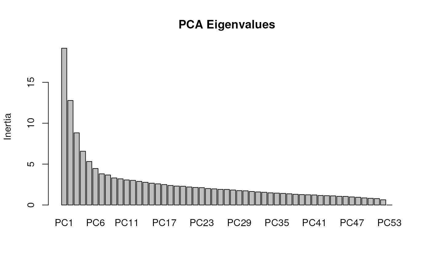
#> Step: R2.adj= 0
#> Call: gen ~ 1
#>
#>                         R2.adjusted
#> <All variables>        0.0202527037
#> + CA_rPCA2             0.0196214014
#> + CA_rPCA3             0.0137427906
#> + CA_rPCA1             0.0009953656
#> <model>                0.0000000000
#> + Condition(PC1 + PC2) 0.0000000000
#>
#>            Df    AIC      F Pr(>F)
#> + CA_rPCA2  1 264.09 2.0407  0.004 **
#> ---
#> Signif. codes:  0 '***' 0.001 '**' 0.01 '*' 0.05 '.' 0.1 ' ' 1
#>
#> Step: R2.adj= 0.0196214
#> Call: gen ~ CA_rPCA2
#>
#>                        R2.adjusted
#> + CA_rPCA3              0.03919420
#> <All variables>         0.02025270
#> + CA_rPCA1              0.01991617
#> <model>                 0.01962140
#> + Condition(PC1 + PC2)  0.01834925
Given this partial RDA, only environmental PC2 is considered significant.
mod_pRDA$anova
#>                   R2.adj Df    AIC      F Pr(>F)
#> + CA_rPCA2      0.019621  1 264.09 2.0407  0.004 **
#> <All variables> 0.020253
#> ---
#> Signif. codes:  0 '***' 0.001 '**' 0.01 '*' 0.05 '.' 0.1 ' ' 1
Now that we have the RDA model, we can discover SNPs that are
outliers. In algatr, this can be done using two different methods to
detect outlier loci, specified by the outlier_method
argument. The first uses Z-scores for outlier detection, and is from Forester
et al. 2018; their code can be found here. The
other method transforms RDA loadings into p-values, and was developed by
Capblancq
et al. 2018 and is further described in Capblancq
& Forester 2021; code developed to run this is associated with
Capblancq and Forester 2021 and can be found here. We
provide brief explanations for each of these methods below.
N.B.: Some researchers may prefer to do MAF filtering and linkage disequilibrium pruning during outlier detection (e.g., Capblancq & Forester 2021). In this case, only one SNP per contig is selected based on the highest loading. The algatr pipeline does this filtering initially when processing genetic data; see data processing vignette for more information.
Identifying outliers using the Z-scores method
To understand how the Z-scores method works to detect outliers, let’s
first take a look at the loadings of SNPs on the first two RDA axes
using the rda_plot() function. This will show us histograms
for each of the selected RDA axes. SNPs that are not associated with
environmental variables will fall in the center of these distributions,
with outliers falling at the edges. The Z-score method works by setting
a Z-score (number of standard deviations) threshold beyond which SNPs
will be considered outliers (see here for
further details).
If we set this value too stringently, we minimize our false positive rate but risk detecting false negatives; if it’s set too high, we increase our false positive rate. Researchers will want to adjust this parameter based on their tolerance for detecting false positives, but also the strength of selection under which outliers are subject to (assuming that SNPs that are more significantly associated with environmental variables are also under stronger selection).
Because only one environmental variable was associated with our genetic data, we only have one resulting RDA axis.
rda_plot(mod_pRDA, axes = "all", binwidth = 20)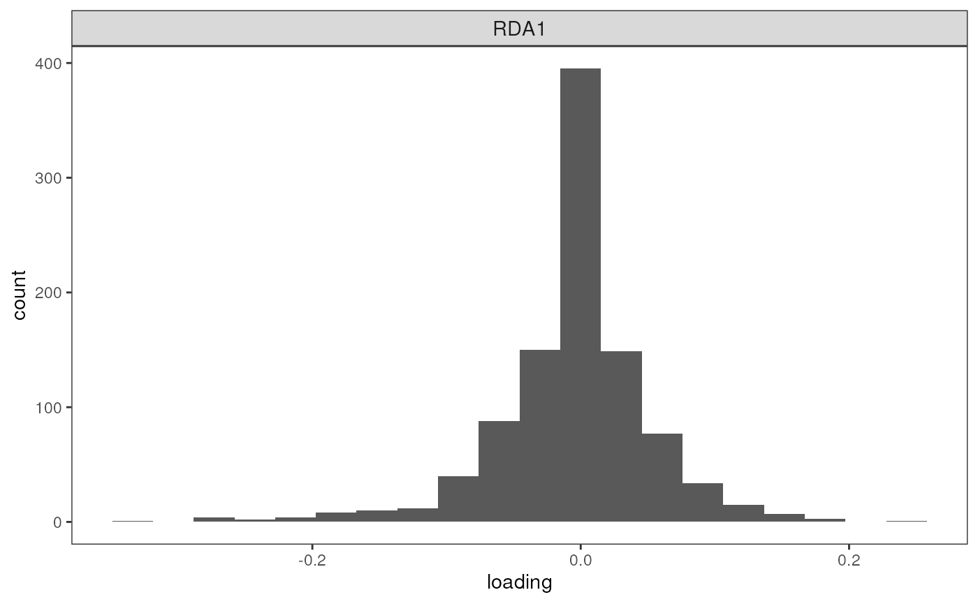
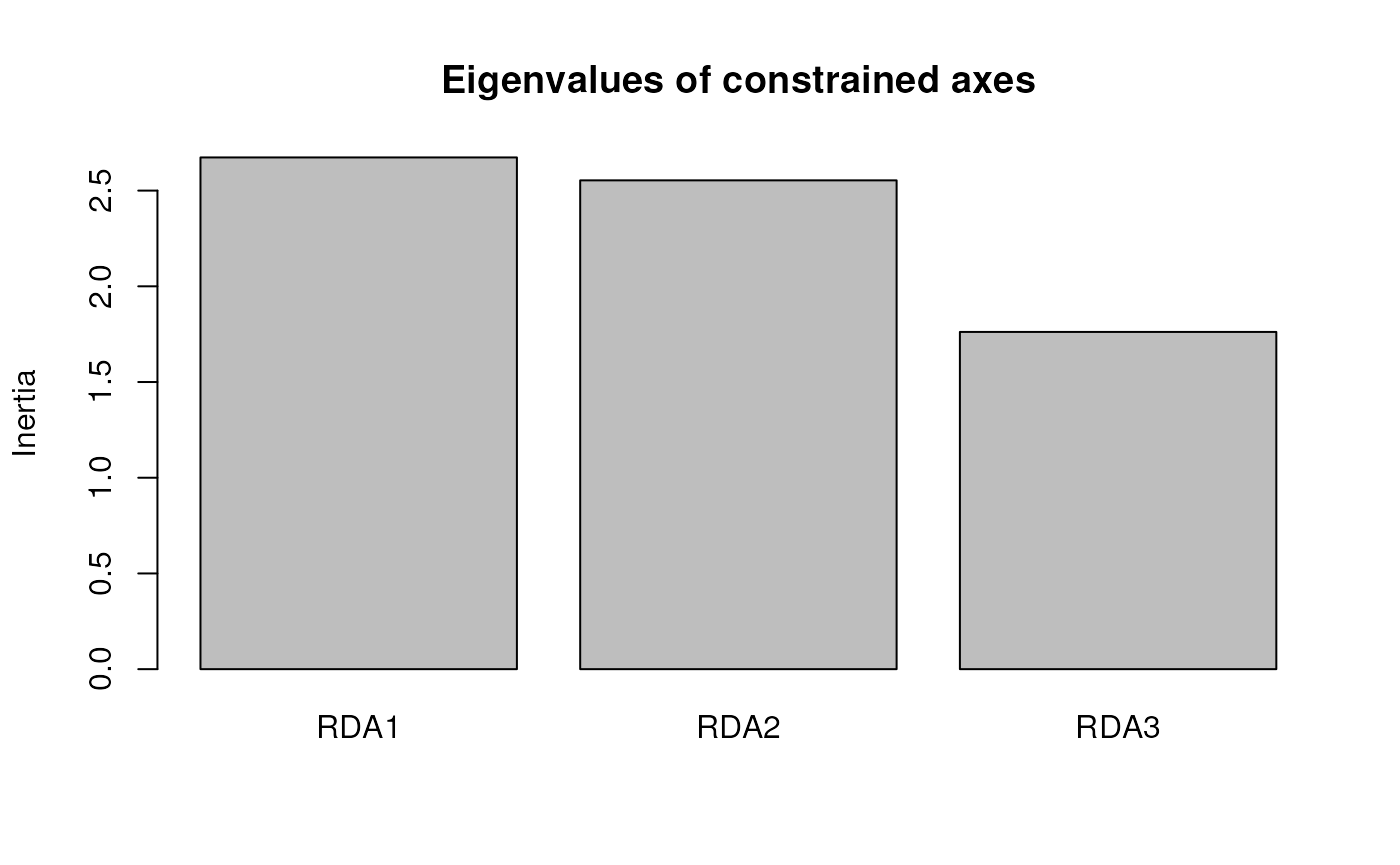
Now, let’s discover outliers with the rda_getoutliers()
function. The method is specified using the outlier_method
argument, and the number of standard deviations to detect outliers is
specified by the z argument; it defaults to 3. The
resulting object is a dataframe containing the SNP name, the RDA axis
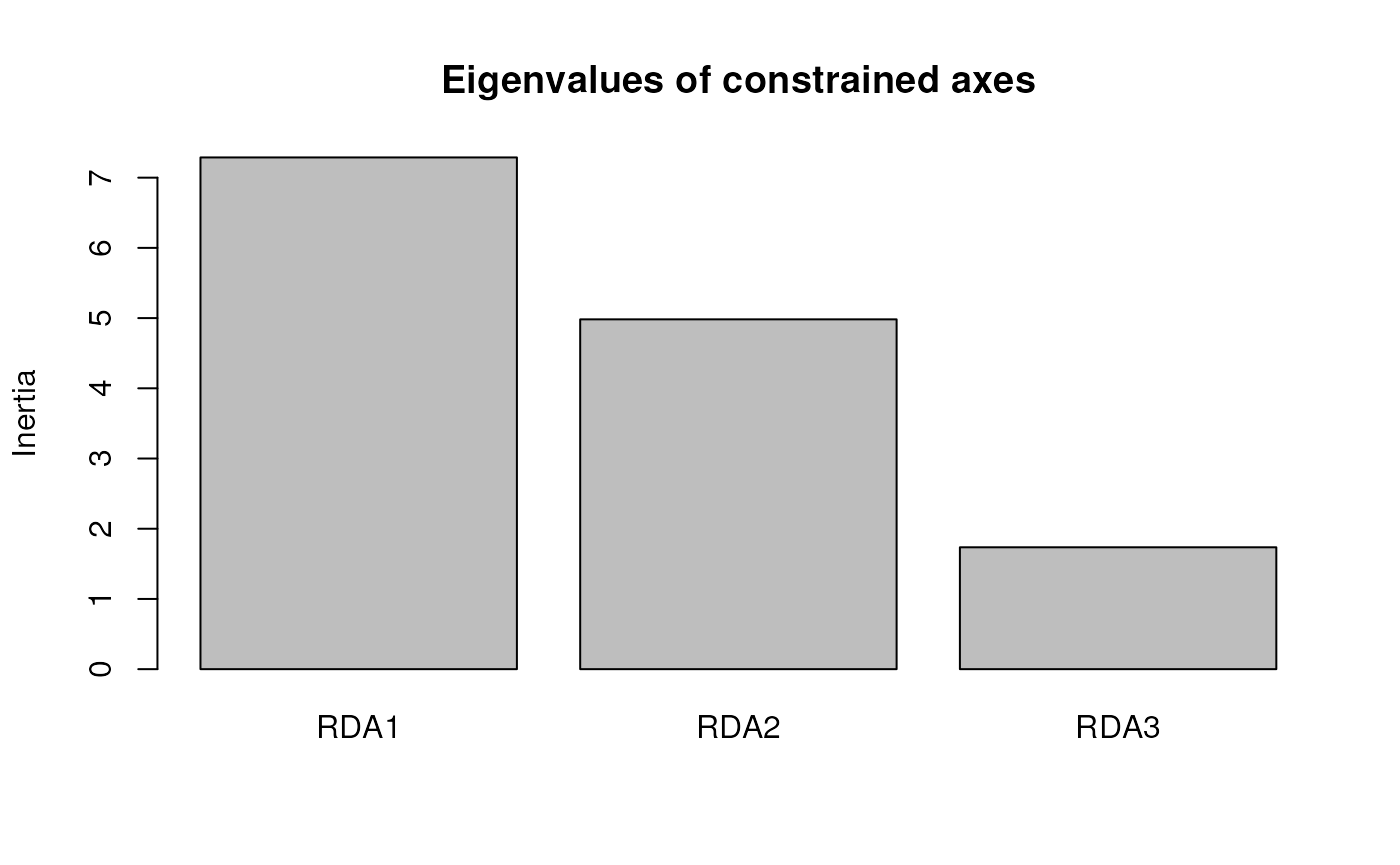
it’s associated with, and the loading along this axis. A screeplot for
the RDA axes is automatically generated (but can be switched off using
the plot argument).
rda_sig_z <- rda_getoutliers(mod_pRDA, naxes = "all", outlier_method = "z", z = 3, plot = FALSE)

# How many outlier SNPs were detected?
length(rda_sig_z$rda_snps)
#> [1] 19
Identifying outliers using the p-value method
Another method to detect outliers is a p-value method wherein rather
than using the loadings along RDA axes to identify extreme outliers (as
with the Z-scores method above), the loadings are transformed into
p-values. To do so, Mahalanobis distances are calculated for each locus,
scaled based on a genomic inflation factor, from which p-values and
q-values can be computed. We then adjust our p-values (based on a false
discovery rate, for example; this adjustment is done using the
p.adjust() function) and subsequently identify outliers
based on a user-specified significance threshold. Rather than detecting
outliers based on a p-value significance threshold, one could also
detect outliers based on q-values (which are also provided as output in
algatr), as is done in Capblancq
et al. 2018 and Capblancq
& Forester 2021. To do so, we would select loci that fall below
a user-specified threshold based on the proportion of false positives we
allow. For example, if we allow 10% or fewer outliers to be false
positives, outliers could be identified based on loci that have q-values
=< 0.1.
Now, let’s detect outliers using this method. To do so, along with
outlier_method, we need to specify p_adj,
which is the method by which p-values are adjusted, as well as
sig, which is our significance threshold. We will also tell
the function not to produce a screeplot.
One limitation of the p-value outlier method is that you cannot
calculate outliers given fewer than two RDA axes (as is the case with
our partial RDA results). So, let’s move forward with this outlier
detection method but using the results from our simple RDA model with
variable selection, mod_best.
rda_sig_p <- rda_getoutliers(mod_best, naxes = "all", outlier_method = "p", p_adj = "fdr", sig = 0.01, plot = FALSE)

# How many outlier SNPs were detected?
length(rda_sig_p$rda_snps)
#> [1] 101
As mentioned above, we could also identify outliers based on
q-values. To do so, we can extract the q-values from the resulting
object from rda_getoutliers().
# Identify outliers that have q-values < 0.1
q_sig <-
  rda_sig_p$rdadapt %>%
  # Make SNP names column from row names
  mutate(snp_names = row.names(.)) %>%
  filter(q.values <= 0.1)

# How many outlier SNPs were detected?
nrow(q_sig)
#> [1] 170
Note the differences between the two methods: using the p-value method, we found many more outlier SNPs than with the Z-scores method (101 vs. 19). Even more outliers were found when only using q-values as a significant threshold (170). We can also see that 19 SNPs were detected using all three methods.
Reduce(intersect, list(
  q_sig$snp_names,
  rda_sig_p$rda_snps,
  rda_sig_z$rda_snps
))
#>  [1] "Locus_517"  "Locus_771"  "Locus_786"  "Locus_945"  "Locus_1247"
#>  [6] "Locus_1263" "Locus_1278" "Locus_1318" "Locus_1374" "Locus_1439"
#> [11] "Locus_1524" "Locus_1801" "Locus_1949" "Locus_2045" "Locus_2338"
#> [16] "Locus_2431" "Locus_2559" "Locus_2665" "Locus_2947"
Visualizing RDA results with rda_plot()
algatr provides options for visualizing RDA results in two ways with
the rda_plot() function: a biplot and a Manhattan plot.
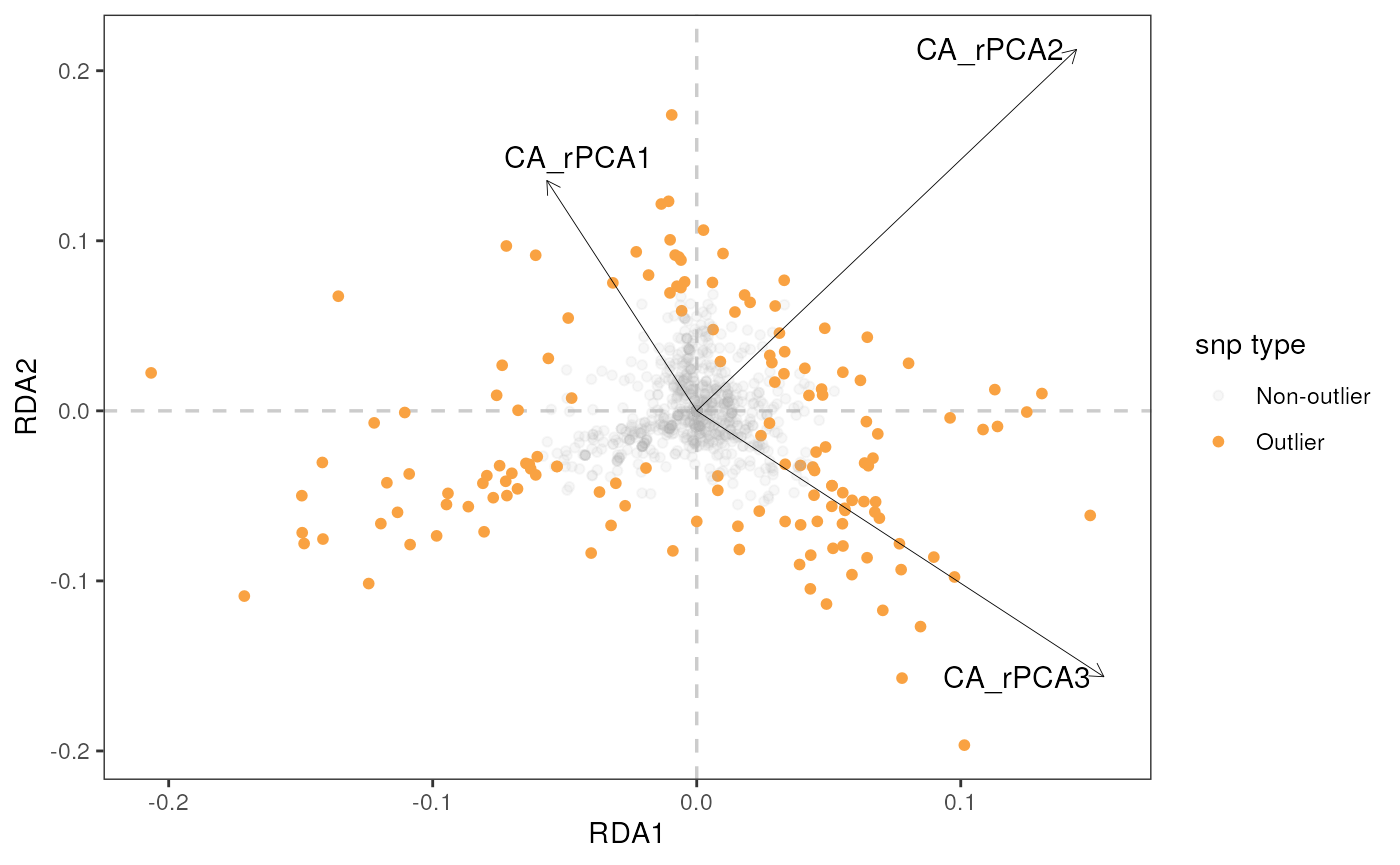
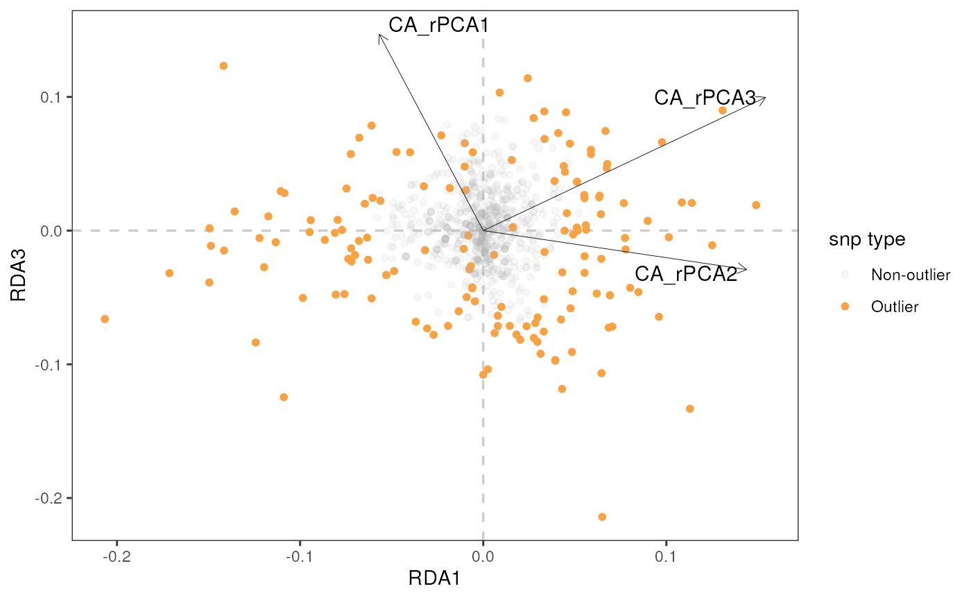
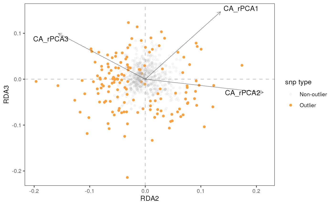
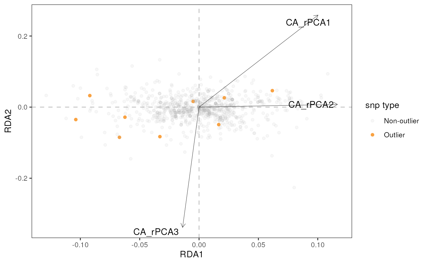
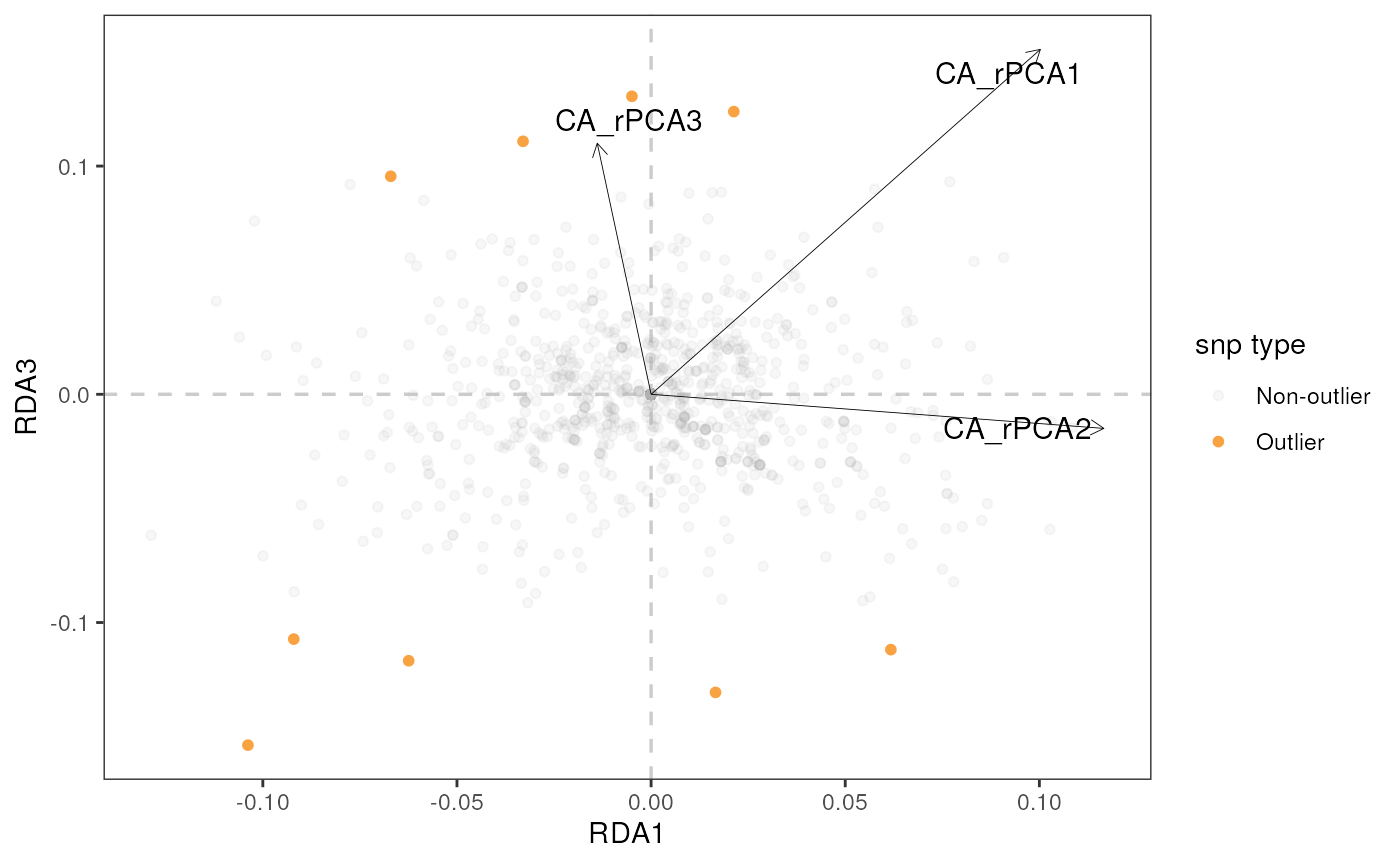
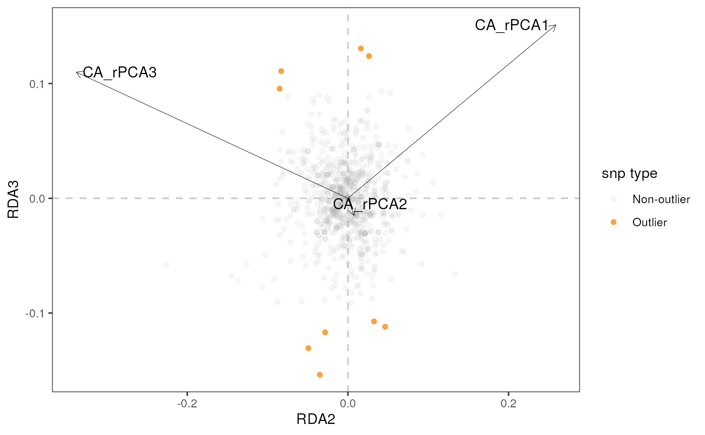
RDA biplot
Let’s build a biplot (or some call it a triplot, since it also shows
loadings of environmental variables) with RDA axes 1 and 2, specified
using the rdaplot argument. In this case, we also need to
specify the number of axes to display using the biplot_axes
argument. The default of rda_plot() is to plot all
variables, regardless of whether they were considered significant or
not.
rda_plot(mod_best, rda_sig_p$rda_snps, biplot_axes = c(1, 2), rdaplot = TRUE, manhattan = FALSE)
#> Warning: Using `size` aesthetic for lines was deprecated in ggplot2 3.4.0.
#> ℹ Please use `linewidth` instead.
#> ℹ The deprecated feature was likely used in the algatr package.
#>   Please report the issue to the authors.
#> This warning is displayed once per session.
#> Call `lifecycle::last_lifecycle_warnings()` to see where this warning was
#> generated.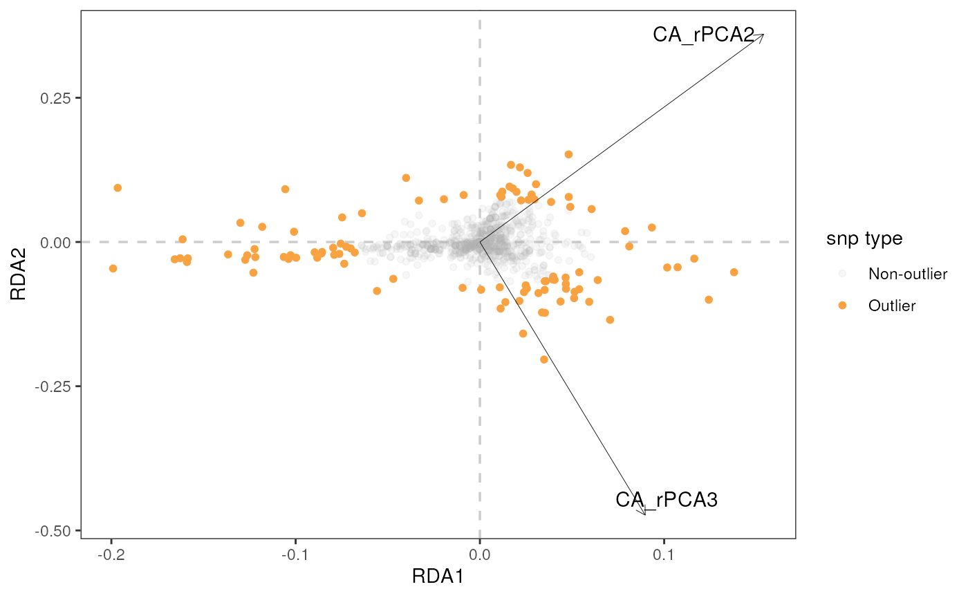
# In the case of our partial RDA, there was only one RDA axis, so a histogram is generated
rda_plot(mod_pRDA, rda_sig_z$rda_snps, rdaplot = TRUE, manhattan = FALSE, binwidth = 0.01)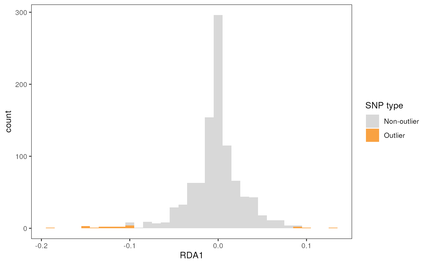
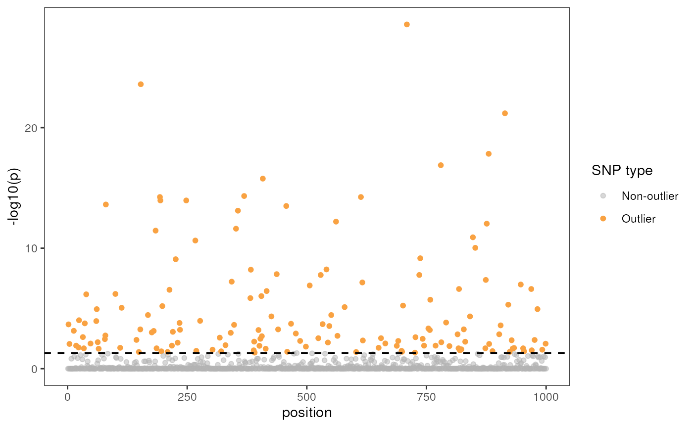
Manhattan plot
Let’s now build a Manhattan plot with a significance level of 0.05
using the manhattan argument; if this is set to TRUE, we
must also provide a significance threshold value using the
sig argument (the default is 0.05). Be aware that outliers
were detected with a different p-value threshold which is why there are
grey points above our threshold line (i.e., data points are colorized
according to the threshold of the model, not the visualization).
rda_plot(mod_best, rda_sig_p$rda_snps, rda_sig_p$pvalues, rdaplot = FALSE, manhattan = TRUE)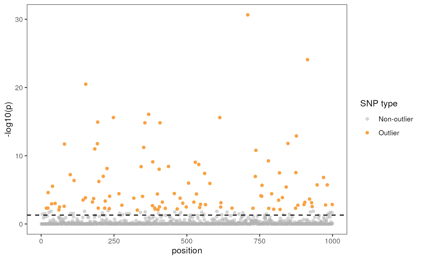
Interpreting RDA results
As discussed in Capblancq & Forester 2021, users should be aware that “statistical selection of variables optimizes variance explained but cannot, by itself, identify the ecological or mechanistic drivers of genetic variation.”
Identifying environmental associations with rda_cor()
and rda_table()
Now that we’ve identified outlier loci, it is useful to be able to
identify how much they correlate to each environmental variable. To do
so, we can run a correlation test of each SNP using
rda_cor() and summarize results in a customizable table
using rda_table().
# Extract genotypes for outlier SNPs
rda_snps <- rda_sig_p$rda_snps
rda_gen <- gen[, rda_snps]

# Run correlation test
cor_df <- rda_cor(rda_gen, env)

# Make a table from these results (displaying only the first 5 rows):
rda_table(cor_df, nrow = 5)
#> Warning: There was 1 warning in `dplyr::mutate()`.
#> ℹ In argument: `dplyr::across(-c(var, snp), round, digits)`.
#> Caused by warning:
#> ! The `...` argument of `across()` is deprecated as of dplyr 1.1.0.
#> Supply arguments directly to `.fns` through an anonymous function instead.
#>
#>   # Previously
#>   across(a:b, mean, na.rm = TRUE)
#>
#>   # Now
#>   across(a:b, \(x) mean(x, na.rm = TRUE))
#> ℹ The deprecated feature was likely used in the algatr package.
#> Please report the issue to the authors.| r | p | snp | var |
|---|---|---|---|
| 0.27 | 0.02 | Locus_125 | CA_rPCA3 |
| 0.39 | 0.00 | Locus_166 | CA_rPCA3 |
| 0.29 | 0.01 | Locus_249 | CA_rPCA2 |
| -0.24 | 0.03 | Locus_263 | CA_rPCA1 |
| 0.27 | 0.02 | Locus_263 | CA_rPCA3 |
# Order by the strength of the correlation
rda_table(cor_df, order = TRUE, nrow = 5)| r | p | snp | var |
|---|---|---|---|
| -0.49 | 0 | Locus_2947 | CA_rPCA2 |
| -0.43 | 0 | Locus_1278 | CA_rPCA2 |
| -0.42 | 0 | Locus_2338 | CA_rPCA3 |
| -0.42 | 0 | Locus_786 | CA_rPCA2 |
| -0.42 | 0 | Locus_1318 | CA_rPCA2 |
# Only retain the top variable for each SNP based on the strength of the correlation
rda_table(cor_df, top = TRUE, nrow = 5)| r | p | snp | var |
|---|---|---|---|
| 0.27 | 0.02 | Locus_125 | CA_rPCA3 |
| 0.39 | 0.00 | Locus_166 | CA_rPCA3 |
| 0.29 | 0.01 | Locus_249 | CA_rPCA2 |
| 0.27 | 0.02 | Locus_263 | CA_rPCA3 |
| 0.28 | 0.01 | Locus_312 | CA_rPCA2 |
# Display results for only one environmental variable
rda_table(cor_df, var = "CA_rPCA2", nrow = 5)| r | p | snp | var |
|---|---|---|---|
| 0.29 | 0.01 | Locus_249 | CA_rPCA2 |
| 0.28 | 0.01 | Locus_312 | CA_rPCA2 |
| 0.27 | 0.02 | Locus_404 | CA_rPCA2 |
| 0.34 | 0.00 | Locus_517 | CA_rPCA2 |
| 0.23 | 0.04 | Locus_612 | CA_rPCA2 |
Running RDA with rda_do_everything()
The algatr package also has an option to run all of the above
functionality in a single function, rda_do_everything().
This function is similar in structure to rda_run(), but
also performs imputation (impute option), can generate
figures, the correlation test table (cortest option;
default is TRUE), and variance partitioning (varpart
option; default is FALSE). Please be aware that the
do_everything() functions are meant to be exploratory. We
do not recommend their use for final analyses unless certain they are
properly parameterized.
The resulting object from rda_do_everything()
contains:
Candidate SNPs:
rda_snpsData frame of environmental associations with outlier SNPs:
cor_dfRDA model specifics:
rda_modOutlier test results:
rda_outlier_testRelevant R-squared values:
rsqANOVA results:
anovaList of all p-values:
pvaluesVariance partitioning results:
varpart
Let’s first run a simple RDA, imputing to the median, with variable selection and the p-value outlier method:
results <- rda_do_everything(liz_vcf, CA_env, liz_coords,
                             impute = "simple",
                             correctGEO = FALSE,
                             correctPC = FALSE,
                             outlier_method = "p",
                             sig = 0.05,
                             p_adj = "fdr",
                             cortest = TRUE,
                             varpart = FALSE
)
| r | p | snp | var |
|---|---|---|---|
| -0.49 | 0 | Locus_2947 | CA_rPCA2 |
| -0.43 | 0 | Locus_1278 | CA_rPCA2 |
| -0.42 | 0 | Locus_2338 | CA_rPCA3 |
| -0.42 | 0 | Locus_786 | CA_rPCA2 |
| -0.42 | 0 | Locus_1318 | CA_rPCA2 |
| -0.42 | 0 | Locus_771 | CA_rPCA2 |
| -0.41 | 0 | Locus_1374 | CA_rPCA2 |
| 0.40 | 0 | Locus_636 | CA_rPCA3 |
| 0.39 | 0 | Locus_1263 | CA_rPCA2 |
| 0.39 | 0 | Locus_166 | CA_rPCA3 |
Now, let’s run a partial RDA, imputing based on 3 sNMF clusters,
correcting for both geography and structure, and instead using the
Z-score method to detect outlier loci, including variance partitioning.
We’ll keep the number of PCs for population structure set to the
default, which is three axes (nPC):
results <- rda_do_everything(liz_vcf, CA_env, liz_coords,
                             impute = "structure",
                             K_impute = 3,
                             model = "full",
                             correctGEO = TRUE,
                             correctPC = TRUE,
                             nPC = 3,
                             varpart = TRUE,
                             outlier_method = "z",
                             z = 3
)
| Variance partitioning | ||||||
| Model | Inertia | R2 | Adjusted R2 | p (>F) | Prop. of explainable variance | Prop. of total variance |
|---|---|---|---|---|---|---|
| Full model | 70.50 | 0.44 | 0.35 | 0.00 | 1.00 | 0.44 |
| Pure enviro. model | 4.80 | 0.03 | 0.01 | 0.01 | 0.07 | 0.03 |
| Pure pop. structure model | 29.48 | 0.18 | 0.16 | 0.00 | 0.42 | 0.18 |
| Pure geography model | 5.43 | 0.03 | 0.01 | 0.00 | 0.08 | 0.03 |
| Confounded variance | 30.80 |
|
|
|
0.44 | 0.19 |
| Total unexplained variance | 89.95 |
|
|
|
|
0.56 |
| Total inertia | 160.45 |
|
|
|
|
1.00 |
| r | p | snp | var |
|---|---|---|---|
| -0.42 | 0.00 | Locus_2338 | CA_rPCA3 |
| -0.35 | 0.00 | Locus_2767 | CA_rPCA1 |
| 0.31 | 0.01 | Locus_2665 | CA_rPCA2 |
| 0.29 | 0.01 | Locus_2053 | CA_rPCA1 |
| -0.29 | 0.01 | Locus_1005 | CA_rPCA1 |
| -0.29 | 0.01 | Locus_1005 | CA_rPCA1 |
| 0.29 | 0.01 | Locus_3058 | CA_rPCA3 |
| 0.28 | 0.01 | Locus_1660 | CA_rPCA2 |
| 0.27 | 0.01 | Locus_469 | CA_rPCA3 |
| 0.27 | 0.02 | Locus_2995 | CA_rPCA2 |
Additional documentation and citations
| Citation/URL | Details | |
|---|---|---|
| Associated literature | Capblancq & Forester 2021; Github repository for code | Paper describing RDA methodology; also provides walkthrough and
description of rdadapt() function |
| Associated literature | Capblancq et al. 2018 | Description of p-value method of detecting outlier loci |
| R package documentation | Oksanen et al. 2022. | algatr uses the rda() and ordiR2step()
functions in the vegan package |
| Associated literature | Forester et al. 2018 | Review of genotype-environment association methods |
| Associated tutorial | Forester et al. | Walkthrough of performing an RDA with the Z-scores outlier detection method |
| Associated vignette | vignette("intro-vegan") |
Introduction to ordination using the vegan package (including using
the rda() function |
| Associated vignette | vignette("partitioning") |
Introduction to variance partitioning in vegan |