LFMM
LFMM_vignette.RmdLatent factor mixed models (LFMM)
# Install required packages
lfmm_packages()If using LFMM, please cite the following: for the LFMM
method, Caye et al. 2019. For the lfmm package, please cite
Jumentier B. (2021). lfmm: Latent Factor Mixed Models. R package version
1.1.
LFMM (Frichot et al. 2013) is a genotype-environment association (GEA) method in which mixed models are used to determine loci that are significantly associated with environmental variables. This method is similar to performing RDA, except that LFMM takes into account – and corrects for – unobserved variables that may confound results (known as latent factors). A good example of a latent factor that we may want to correct for prior to examining environment-associated loci is population structure.
There are a variety of ways to determine the best number of latent factors in LFMM (which are called K values, although these are not the same as TESS K values). algatr provides the option to test using four such methods: (1) Tracy-Widom test; (2) quick elbow test (i.e., scree test); (3) using the clustering algorithm from TESS (i.e., determining latent factors corresponding to some measure of population structure); and (4) K-means clustering. We will explore each of these, and compare results, in this vignette.
Importantly, as with RDA, LFMM cannot take in missing values.
Imputation based on the per-site median is commonly performed, but there
are several other ways researchers can deal with missing values. For
example, algatr contains the str_impute() function to
impute missing values based on population structure using the
LEA::impute() function. However, here, we’ll impute on the
median, but strongly urge researchers to use extreme caution when using
this form of simplistic imputation. We mainly provide code to impute on
the median for testing datasets and highly discourage its use in further
analyses (please use str_impute() instead!).
To perform an LFMM analysis (Caye et
al. 2019), algatr uses the lfmm package (see here for details).
Despite its name, this package implements the LFMM2 method, which is
similar to the original LFMM algorithm, but is computationally faster.
The LEA package (Frichot &
Francois 2015) also provides a wrapper for lfmm2 using the
lfmm2() function.
Read in and process data files
To run LFMM, we will need a genotype dosage matrix and environmental
values extracted at sampling coordinates. Let’s load the example
dataset, convert the vcf to a dosage matrix using the
vcf_to_dosage() function, and extract environmental data
for our sampling coordinates from our environmental raster stack
(CA_env).
load_algatr_example()
#>
#> ---------------- example dataset ----------------
#>
#> Objects loaded:
#> *liz_vcf* vcfR object (1000 loci x 53 samples)
#> *liz_gendist* genetic distance matrix (Plink Distance)
#> *liz_coords* dataframe with x and y coordinates
#> *CA_env* RasterStack with example environmental layers
#>
#> -------------------------------------------------
#>
#>
# Convert vcf to dosage matrix
gen <- vcf_to_dosage(liz_vcf)
#> Loading required namespace: vcfR
#> Loading required namespace: adegenet
# Also, our code assumes that sample IDs from gendist and coords are the same order; be sure to check this before moving forward!
env <- raster::extract(CA_env, liz_coords)
As mentioned above, LFMM requires that your genotype matrix contains no missing values. Let’s impute missing values based on the per-site median. N.B.: this type of simplistic imputation is strongly not recommended for downstream analyses and is used here for example’s sake!
# Are there NAs in the data?
gen[1:5, 1:5]
#>        Locus_10 Locus_15 Locus_22 Locus_28 Locus_32
#> ALT3          0        0        0        0        0
#> BAR360        0        0        0       NA        0
#> BLL5          0       NA        0        0       NA
#> BNT5          0        0       NA       NA        0
#> BOF1          0       NA       NA       NA       NA
gen <- simple_impute(gen)
# Check that NAs are gone
gen[1:5, 1:5]
#>        Locus_10 Locus_15 Locus_22 Locus_28 Locus_32
#> ALT3          0        0        0        0        0
#> BAR360        0        0        0        0        0
#> BLL5          0        0        0        0        0
#> BNT5          0        0        0        0        0
#> BOF1          0        0        0        0        0
Determining the number of latent factors using
select_K()
LFMM requires a user to define the number of latent factors (K
values). algatr provides options to perform four types of K selection
using the K_selection parameter within the
select_K() function:
K_selection = "tracy_widom": A Tracy-Widom test is performed. Briefly, this method finds significant eigenvalues of a matrix after performing a PCA. This argument uses thetw()function within the AssocTests package, and also requires a user to provide thecriticalpoint, which corresponds to the significance level. Significance levels of alpha=0.05, 0.01, 0.005, or 0.001 correspond to critical point values of 0.9793, 2.0234, 2.4224, or 3.2724, respectively. The default significance level is 0.01, so the default for thecriticalpointparameter is 2.0234. The Tracy-Widom test is also the default method for theselect_K()function.K_selection = "quick_elbow": A “quick elbow” is found automatically, which refers to a large percent drop in eigenvalues given a variance below 5% for each principal component (essentially the same as a scree test). The code to determine a quick elbow is adapted from that developed by Nicholas Cooper here. This argument requires users to set the threshold that defines whether a principal component explains ‘much’ of the variance using thelowargument, and also the maximum percentage of the variance to capture before the elbow (i.e., the cumulative sum to PC ‘n’) using themax.pcargument. The default forlowis 0.08, and the default formax.pcis 0.90.K_selection = "tess": The automatic K selection is performed after running TESS. This method minimizes the slope of the line that connects cross-entropy scores between K values. This approach is described here. This argument requires users to provide coordinates (coords) and set the range of K values to test (Kvals; defaults to 1:10).-
K_selection = "find_clusters": Uses K-means clustering to detect the number of clusters that best describe the data; this uses thefind.clusters()function in the adegenet package. For this method, the data are first transformed using a PCA, after which successive K-means clustering is run with an increasing number of K values. The “best” K is selected using the"diffNgroup” criterion in adegenet’sfind.clustersfunction. algatr’s"find_clusters"argument requires users to set several parameters for both the PCA and the K-means clustering steps:The user must specify the minimum amount of the total variance to be preserved by the retained axes using the
perc.pcaargument. The default for this argument is 90%.The maximum number of clusters to be tested using the
max.n.clustparameter; the default for this is 10.
There are more options within the find.clusters function
in adegenet, but we’ve chosen to include only some of them in algatr
(e.g., the pca.select argument is set to
"percVar"). Please refer to the adegenet documentation for
further information.
Let’s see how the above methods compare to one another in terms of
how K values compare. Regardless of the K selection that’s done, a user
must provide a dosage matrix (gen) and the K selection
procedure they would like to perform (K_selection).
# Keep relevant params but retain default values for them
select_K(gen, K_selection = "tracy_widom", criticalpoint = 2.0234) # 6
#> [1] 6

select_K(gen, K_selection = "quick_elbow", low = 0.08, max.pc = 0.90) # 3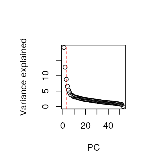
#> [1] 3

select_K(gen, K_selection = "tess", coords = liz_coords, Kvals = 1:10) # 3
#> == Computing spectral decomposition of graph laplacian matrix: done
#> ==Main loop with 1 threads: done
#> == Computing spectral decomposition of graph laplacian matrix: done
#> ==Main loop with 1 threads: done
#> == Computing spectral decomposition of graph laplacian matrix: done
#> ==Main loop with 1 threads: done
#> == Computing spectral decomposition of graph laplacian matrix: done
#> ==Main loop with 1 threads: done
#> == Computing spectral decomposition of graph laplacian matrix: done
#> ==Main loop with 1 threads: done
#> == Computing spectral decomposition of graph laplacian matrix: done
#> ==Main loop with 1 threads: done
#> == Computing spectral decomposition of graph laplacian matrix: done
#> ==Main loop with 1 threads: done
#> == Computing spectral decomposition of graph laplacian matrix: done
#> ==Main loop with 1 threads: done
#> == Computing spectral decomposition of graph laplacian matrix: done
#> ==Main loop with 1 threads: done
#> == Computing spectral decomposition of graph laplacian matrix: done
#> ==Main loop with 1 threads: done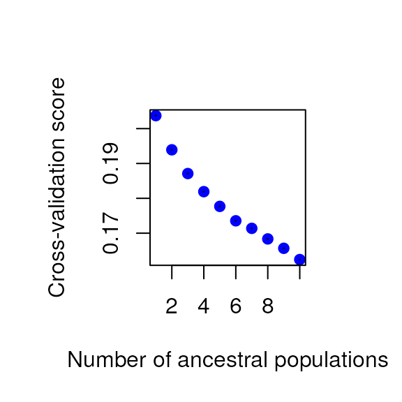
#> [1] 3

select_K(gen, K_selection = "find_clusters", perc.pca = 90, max.n.clust = 10) # 4
#> [1] 3
As you can see, the K selection method has quite an effect on the best number of latent factors discovered in the data. For this vignette, let’s move forward with the best K from the default method (Tracy-Widom test), which means K = 6.
Comparing different LFMM methods with lfmm_run()
The main function in algatr that runs LFMM is
lfmm_run(). This function requires that users provide the
dosage matrix (gen), the extracted environmental variables
(env), the number of latent factors (K), and
the LFMM method (lfmm_method).
Importantly, LFMM can be performed using two main methods
("lasso" or "ridge"), which primarily differ
in the penalized loss functions that are incorporated into the
least-squares minimization and are specified using the
lfmm_method argument. The least-squares minimization is how
statistical significance is determined for SNPs being associated with
environmental variables. The primary difference between the two methods
is that the ridge method minimizes the problem with an L^2 penalty,
whereas the lasso method minimizes with an L^1 penalty. According to Caye
& François 2017, a user would want to select the lasso method
(i.e., L^1-norm) to induce “sparsity on the fixed effects, and
corresponds to the prior information that not all response variables may
be associated with the variables of interest. More specifically, the
prior implies that a limited number of rows of the effect size matrix B
are effectively non-zero.” The ridge penalty is further described in Caye et
al. 2019.
One other argument to be aware of within lfmm_run() is
the adjustment of p-values, specified using p_adj. There
are two options for p_adj: "fdr", which
adjusts calibrated p-values based on the false discovery rate (the
default). Other options for p-value adjustment can be found within the
p.adjust() function in the stats package.
Finally, the last argument to be aware of within
lfmm_run() is calibrate, which calibrates
p-values based on resulting z-scores. There are two options for this
argument: "gif" (the default), and
"median+MAD". From the LFMM documentation: “If the”gif”
option is set (default), significance values are calibrated by using the
genomic control method. Genomic control uses a robust estimate of the
variance of z-scores called “genomic inflation factor”. If the
“median+MAD” option is set, the pvalues are calibrated by computing the
median and MAD of the zscores. If NULL, the pvalues are not
calibrated.”
Now that we’ve identified the number of latent factors to provide in our model, let’s run LFMM using both ridge and lasso penalties with default settings (i.e., FDR p-value adjustment and the “gif” calibration).
ridge_results <- lfmm_run(gen, env, K = 6, lfmm_method = "ridge")
lasso_results <- lfmm_run(gen, env, K = 6, lfmm_method = "lasso")
The results object from lfmm_run() contains 5
elements:
lfmm_snps: a list of candidate SNPs that are statistically significantly associated with environmental variables, including all relevant information pertaining to the LFMM analysis (e.g., p-values, fixed effects, etc.)df: all of the SNPs and their associations, including all relevant information pertaining to the LFMM analysismodel: parameters of the LFMM model, including matrices B, U, and Vlfmm_test_result: results from association testingK: the number of latent factors that LFMM was run using (in our case, 6)
Visualizing LFMM results
There are three main ways we can visualize the results from our LFMM
analysis. Each of these is automatically produced by
lfmm_run(), but you can produce them individually as well
with the functions below.
-
lfmm_table(): Build a table with each SNP and its association (and p-value) with each environmental variable. This function allows for quite a bit of customization in terms of what is displayed:sig: the significance threshold (alpha value)sig_only: whether to only display SNPs above the significance thresholdtop: if there are SNPs that are significantly associated with multiple environmental variables, only display the top association (i.e., variable with the maximum B value)order: whether to order the SNPs in descending order based on their B value, otherwise they will be ordered based on environmental variablevar: only display SNPs associated with one environmental variablenrow: the number of rows to displaydigits: the number of decimal places to includefootnotes: whether to include footnotes describing the variables displayedp_adj: whether p-values were adjusted inlfmm_run()
lfmm_qqplot(): Build a QQ-plot (quantile-quantile plot) which plots expected quantiles (percentiles) against p-values.lfmm_manhattanplot(): Build a Manhattan plot with defined significance threshold.
Building a table of SNP associations with
lfmm_table()
Let’s see what the top candidate SNPs were for each of our LFMM runs:
# Build tables for each of our LFMM runs, displaying only significant SNPs and ordering according to effect size (B)
lfmm_table(lasso_results$df, order = TRUE)
#> Warning: There was 1 warning in `dplyr::mutate()`.
#> ℹ In argument: `dplyr::across(-c(var, snp), round, digits)`.
#> Caused by warning:
#> ! The `...` argument of `across()` is deprecated as of dplyr 1.1.0.
#> Supply arguments directly to `.fns` through an anonymous function instead.
#>
#>   # Previously
#>   across(a:b, mean, na.rm = TRUE)
#>
#>   # Now
#>   across(a:b, \(x) mean(x, na.rm = TRUE))
#> ℹ The deprecated feature was likely used in the algatr package.
#> Please report the issue to the authors.| snp | variable | B1 | z-score | p-value | calibrated z-score | calibrated p-value | adjusted p-value |
|---|---|---|---|---|---|---|---|
| Locus_2338 | CA_rPCA3 | -0.26 | -4.44 | 0 | 19.19 | 0 | 0.01 |
| Locus_125 | CA_rPCA3 | 0.18 | 3.80 | 0 | 14.09 | 0 | 0.04 |
| Locus_859 | CA_rPCA3 | 0.18 | 3.80 | 0 | 14.09 | 0 | 0.04 |
| Locus_249 | CA_rPCA2 | 0.14 | 4.95 | 0 | 16.78 | 0 | 0.04 |
| Locus_1051 | CA_rPCA3 | 0.09 | 3.80 | 0 | 14.09 | 0 | 0.04 |
| Locus_562 | CA_rPCA2 | -0.05 | -4.74 | 0 | 15.42 | 0 | 0.04 |
| 1 LFMM effect size | |||||||
lfmm_table(ridge_results$df, order = TRUE)| snp | variable | B1 | z-score | p-value | calibrated z-score | calibrated p-value | adjusted p-value |
|---|---|---|---|---|---|---|---|
| Locus_2338 | CA_rPCA3 | -0.29 | -5.25 | 0 | 25.50 | 0 | 0.00 |
| Locus_125 | CA_rPCA3 | 0.17 | 4.08 | 0 | 15.43 | 0 | 0.02 |
| Locus_859 | CA_rPCA3 | 0.17 | 4.08 | 0 | 15.43 | 0 | 0.02 |
| Locus_2947 | CA_rPCA2 | -0.13 | -7.49 | 0 | 38.03 | 0 | 0.00 |
| Locus_512 | CA_rPCA3 | 0.13 | 3.85 | 0 | 13.71 | 0 | 0.03 |
| Locus_2014 | CA_rPCA3 | 0.13 | 3.85 | 0 | 13.71 | 0 | 0.03 |
| Locus_1524 | CA_rPCA2 | -0.12 | -4.84 | 0 | 15.89 | 0 | 0.00 |
| Locus_249 | CA_rPCA2 | 0.12 | 5.92 | 0 | 23.78 | 0 | 0.00 |
| Locus_2338 | CA_rPCA2 | -0.11 | -4.00 | 0 | 10.84 | 0 | 0.03 |
| Locus_2133 | CA_rPCA2 | -0.10 | -6.45 | 0 | 28.25 | 0 | 0.00 |
| Locus_831 | CA_rPCA2 | -0.10 | -5.07 | 0 | 17.46 | 0 | 0.00 |
| Locus_2669 | CA_rPCA2 | -0.09 | -5.29 | 0 | 18.98 | 0 | 0.00 |
| Locus_2703 | CA_rPCA2 | 0.09 | 4.02 | 0 | 10.97 | 0 | 0.03 |
| Locus_1278 | CA_rPCA2 | -0.09 | -5.48 | 0 | 20.33 | 0 | 0.00 |
| Locus_786 | CA_rPCA2 | -0.09 | -4.31 | 0 | 12.61 | 0 | 0.01 |
| Locus_1318 | CA_rPCA2 | -0.09 | -6.51 | 0 | 28.74 | 0 | 0.00 |
| Locus_1051 | CA_rPCA3 | 0.09 | 4.08 | 0 | 15.43 | 0 | 0.02 |
| Locus_2045 | CA_rPCA2 | -0.08 | -5.72 | 0 | 22.21 | 0 | 0.00 |
| Locus_1319 | CA_rPCA2 | -0.08 | -5.59 | 0 | 21.15 | 0 | 0.00 |
| Locus_1745 | CA_rPCA2 | -0.08 | -5.59 | 0 | 21.15 | 0 | 0.00 |
| Locus_2670 | CA_rPCA2 | -0.08 | -6.91 | 0 | 32.38 | 0 | 0.00 |
| Locus_138 | CA_rPCA2 | 0.08 | 4.66 | 0 | 14.73 | 0 | 0.01 |
| Locus_903 | CA_rPCA2 | -0.07 | -5.06 | 0 | 17.39 | 0 | 0.00 |
| Locus_870 | CA_rPCA2 | -0.06 | -5.75 | 0 | 22.40 | 0 | 0.00 |
| Locus_2426 | CA_rPCA2 | -0.06 | -5.75 | 0 | 22.40 | 0 | 0.00 |
| Locus_2699 | CA_rPCA2 | -0.06 | -5.75 | 0 | 22.40 | 0 | 0.00 |
| Locus_2145 | CA_rPCA2 | -0.06 | -3.95 | 0 | 10.55 | 0 | 0.04 |
| Locus_2770 | CA_rPCA2 | -0.06 | -4.11 | 0 | 11.47 | 0 | 0.02 |
| Locus_562 | CA_rPCA2 | -0.06 | -7.05 | 0 | 33.70 | 0 | 0.00 |
| Locus_1414 | CA_rPCA2 | 0.06 | 3.90 | 0 | 10.30 | 0 | 0.04 |
| Locus_974 | CA_rPCA2 | -0.04 | -5.59 | 0 | 21.15 | 0 | 0.00 |
| Locus_1254 | CA_rPCA2 | -0.04 | -5.59 | 0 | 21.15 | 0 | 0.00 |
| Locus_3116 | CA_rPCA2 | -0.04 | -5.59 | 0 | 21.15 | 0 | 0.00 |
| Locus_2421 | CA_rPCA2 | -0.04 | -4.38 | 0 | 13.04 | 0 | 0.01 |
| Locus_637 | CA_rPCA2 | 0.04 | 4.22 | 0 | 12.06 | 0 | 0.02 |
| 1 LFMM effect size | |||||||
As you can see from the above, the penalty chosen makes quite a bit
of difference in terms of how many significant SNPs are found (only 6
with the lasso method, but 35 with the ridge method). However, the three
SNPs with the largest effect size are the same between the two methods
(loci 2338, 125, and 859), and the effect sizes and p-values are
comparable. The tables also contain columns for calibrated z-score,
calibrated p-values, and adjusted p-values. Recall that adjusted
p-values are calculated based on setting the p_adj
argument; in our case, these are adjusted based on the false discovery
rate, which is why they differ from non-adjusted p-values (i.e., values
in the p-value column).
Let’s only look at SNPs significantly associated with the PCA2 environmental variable from the lasso method:
lfmm_table(lasso_results$df, order = TRUE, var = "CA_rPCA2")| snp | variable | B1 | z-score | p-value | calibrated z-score | calibrated p-value | adjusted p-value |
|---|---|---|---|---|---|---|---|
| Locus_249 | CA_rPCA2 | 0.14 | 4.95 | 0 | 16.78 | 0 | 0.04 |
| Locus_562 | CA_rPCA2 | -0.05 | -4.74 | 0 | 15.42 | 0 | 0.04 |
| 1 LFMM effect size | |||||||
# Be aware that if significant SNPs < nrow, function will return NULL object
# lfmm_table(lasso_results$df, sig_only = FALSE, order = FALSE, nrow=10)

# Similarly, the same will occur if you try to specify a variable that is not significantly associated with a SNP
# lfmm_table(lasso_results$df, sig_only = TRUE, var = "CA_rPCA1")
Building a QQplot with lfmm_qqplot()
A QQplot plots theoretical quantiles against p-value quantiles, providing a way to visualize the normality of the test significance values. The line that is plotted runs through the intercept and has a slope of 1. The points should ideally fall along this reference line:
lfmm_qqplot(lasso_results$df)
#> Warning: Removed 414 rows containing non-finite outside the scale range
#> (`stat_qq()`).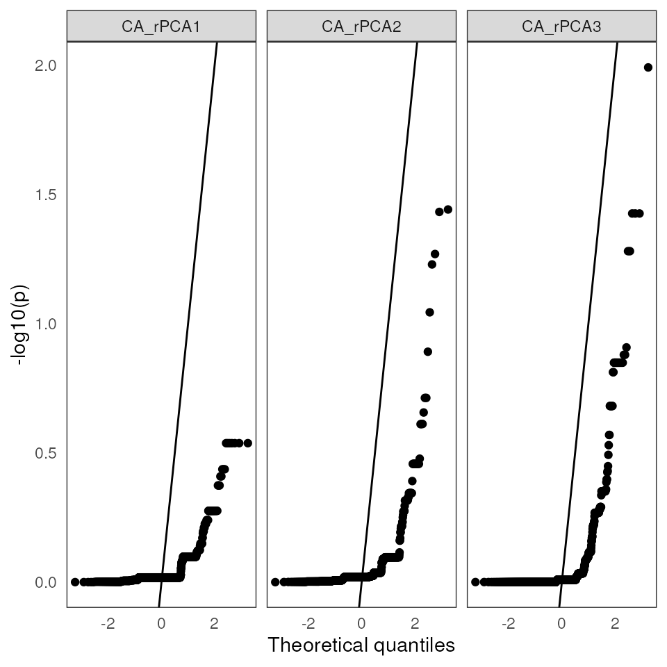
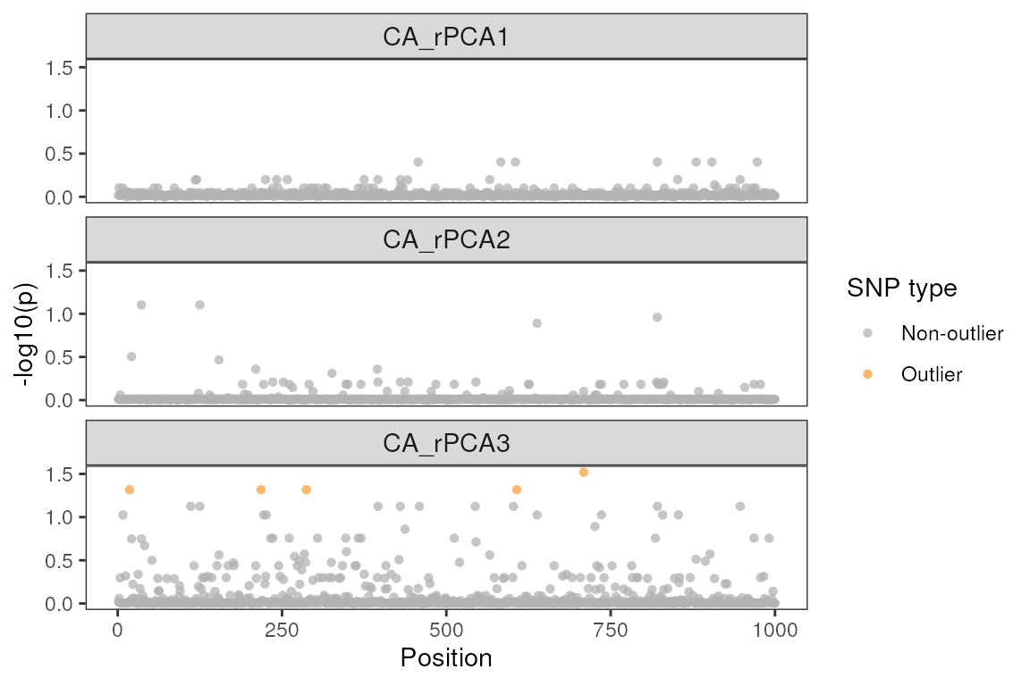
Building a Manhattan plot using
lfmm_manhattanplot()
Manhattan plots are helpful ways to visualize the position of the outlier SNPs across the genome, as well as how much they exceed a user-specified significance threshold for each environmental variable.
# As displayed in our table from above, only six SNPs are visible on the lasso method plots as outliers:
lfmm_manhattanplot(lasso_results$df, sig = 0.05)
#> Warning: Removed 414 rows containing missing values or values outside the scale range
#> (`geom_point()`).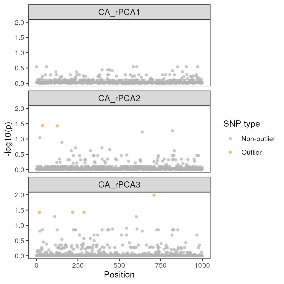
For the ridge method LFMM run, we can see that there are (a) more outliers than the lasso method above, and (b) the majority of these outliers are associated with environmental PC2.
lfmm_manhattanplot(ridge_results$df, sig = 0.05)
#> Warning: Removed 414 rows containing missing values or values outside the scale range
#> (`geom_point()`).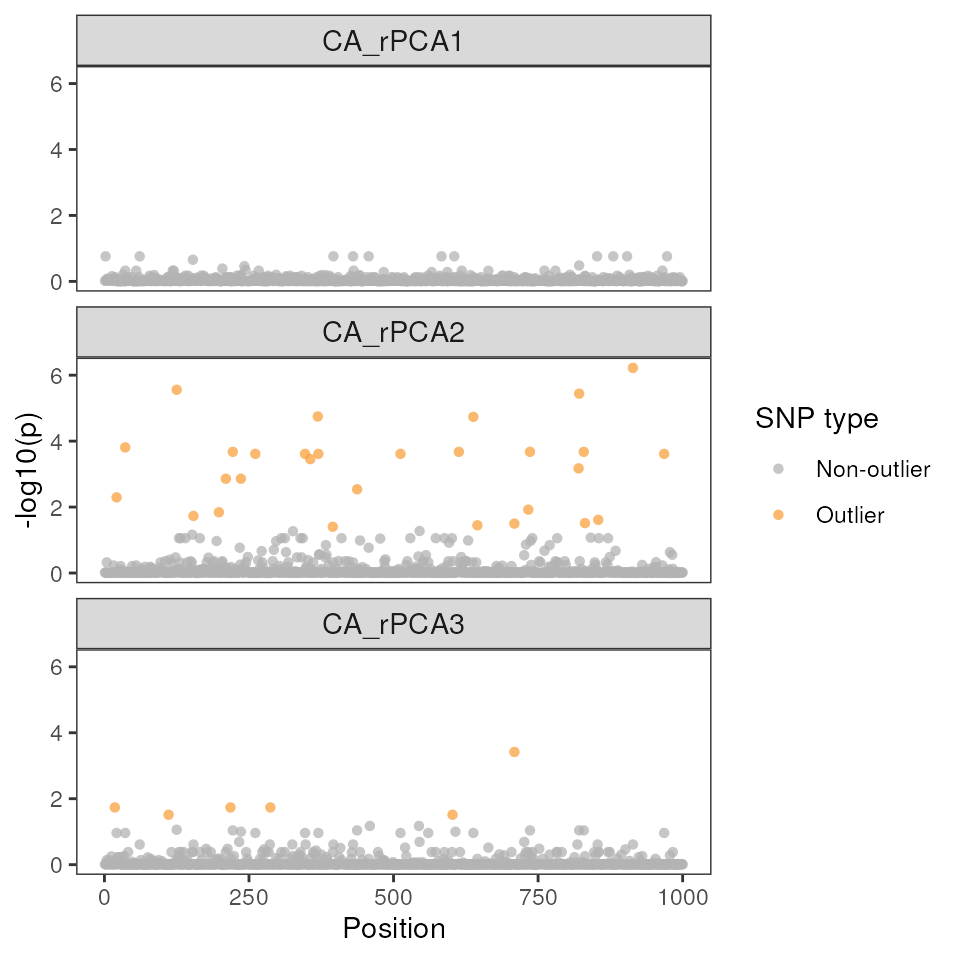
Running LFMM with lfmm_do_everything()
The algatr package also has an option to run all of the above
functionality in a single function, lfmm_do_everything().
This function will automatically extract relevant values from our
environmental layers given our coordinate data; it will also
automatically convert a vcf object to a dosage matrix for us and impute
missing values if present. The output looks the same as the output from
lfmm_run() above, and plots will be automatically produced.
Please be aware that the do_everything() functions
are meant to be exploratory. We do not recommend their use for final
analyses unless certain they are properly parameterized.
lfmm_full_everything <- lfmm_do_everything(liz_vcf, CA_env, liz_coords,
                              impute = "structure",
                              K_impute = 3,
                              lfmm_method = "lasso",
                              K_selection = "tracy_widom")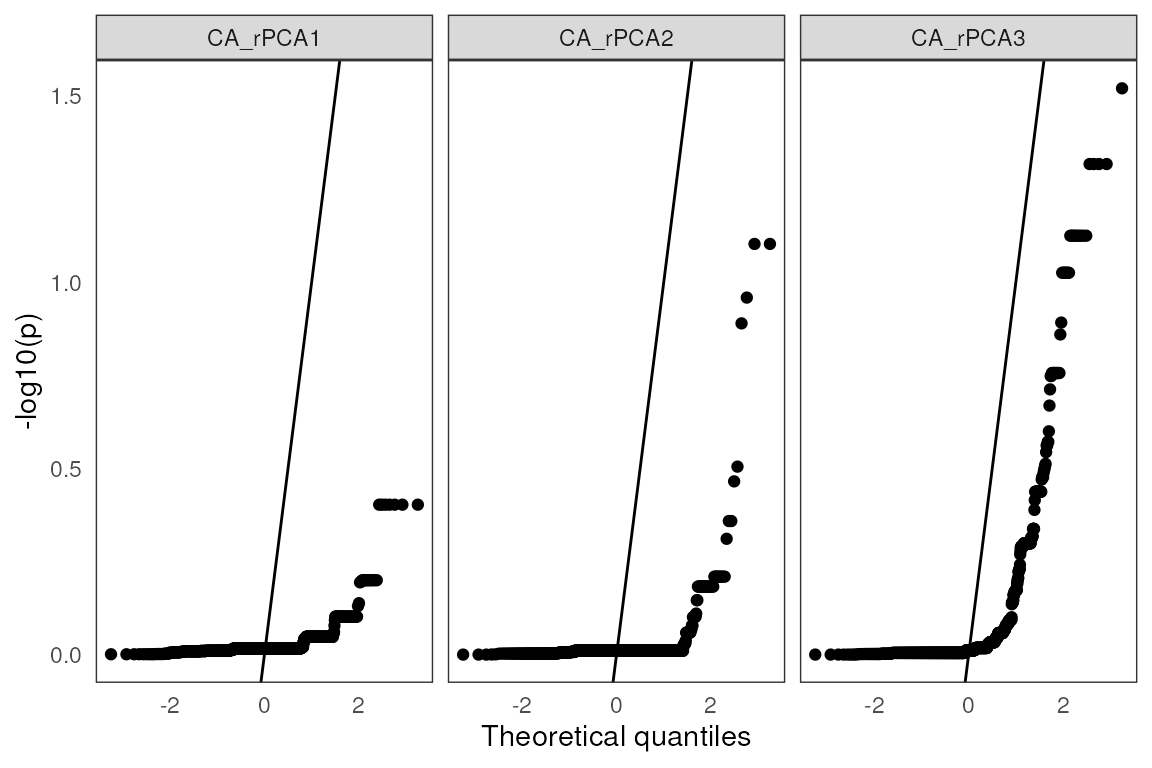
| snp | variable | B1 | z-score | p-value | calibrated z-score | calibrated p-value | adjusted p-value |
|---|---|---|---|---|---|---|---|
| Locus_2338 | CA_rPCA3 | -0.26 | -4.44 | 0 | 17.50 | 0 | 0.02 |
| Locus_249 | CA_rPCA2 | 0.15 | 5.12 | 0 | 17.18 | 0 | 0.02 |
| Locus_2133 | CA_rPCA2 | -0.10 | -4.65 | 0 | 14.18 | 0 | 0.04 |
| Locus_2670 | CA_rPCA2 | -0.08 | -4.88 | 0 | 15.61 | 0 | 0.02 |
| Locus_562 | CA_rPCA2 | -0.06 | -5.04 | 0 | 16.62 | 0 | 0.02 |
| 1 LFMM effect size | |||||||
Additional documentation and citations
| Citation/URL | Details | |
|---|---|---|
| Main manuscript describing method | Caye et al. 2019; see here for documentation | Paper and code describing LFMM2 |
| Associated literature | Frichot et al. 2013 | Paper describing LFMM |
| Associated code | Wang et al. 2020 | algatr performs a Tracy-Widom test using the tw()
function in the AssocTests package |
| Associated code | Blog post on automatic K selection | algatr’s automatic K selection code |
| Additional code | Frichot & Francois 2015 | The LEA package provides wrapper functions for LFMM (using the
lfmm2() function |
Retrieve LFMM’s vignette:
vignette("lfmm")
#> starting httpd help server ... done