Genetic data processing
data_processing_vignette.RmdProcessing genomic data files
# Install required packages
data_processing_packages()For landscape genomic analyses, we first need to process our input data files in various ways. It is important to understand what this data processing is doing, so in this vignette, we’ll do the following:
vcf_to_dosage()to convert a vcf file to a dosage matrixstr_impute()andsimple_impute()to impute missing data in two different waysld_prune()to prune variants that are in linkage disequilibrium with one another; this primarily uses thesnpgdsLDpruning()function within the SNPRelate package (Zheng et al. 2012; see here for further information)
Converting a vcf to a dosage matrix with
vcf_to_dosage()
Recall the way genotypes are encoded within a vcf: "0/0"
denotes individual is homozygous for the reference allele,
"0/1" for heterozygote, and "1/1" for a
homozygote for the alternate allele; NA is missing
data.
# Load the example data
load_algatr_example()
#>
#> ---------------- example dataset ----------------
#>
#> Objects loaded:
#> *liz_vcf* vcfR object (1000 loci x 53 samples)
#> *liz_gendist* genetic distance matrix (Plink Distance)
#> *liz_coords* dataframe with x and y coordinates
#> *CA_env* RasterStack with example environmental layers
#>
#> -------------------------------------------------
#>
#>

# Look at genotypes for five individuals at eight sites:
liz_vcf@gt[1:8, 2:6]
#>      ALT3  BAR360 BLL5  BNT5  BOF1
#> [1,] "0/0" "0/0"  "0/0" "0/0" "0/0"
#> [2,] "0/0" "0/0"  NA    "0/0" NA
#> [3,] "0/0" "0/0"  "0/0" NA    NA
#> [4,] "0/0" NA     "0/0" NA    NA
#> [5,] "0/0" "0/0"  NA    "0/0" NA
#> [6,] NA    "0/0"  "0/0" "0/0" NA
#> [7,] NA    "0/0"  "0/0" NA    "0/0"
#> [8,] "1/1" "1/1"  "0/1" "0/0" "0/0"
A dosage matrix contains each row as an individual (unlike a vcf) and
each column as a site. Importantly, genotypes are now encoded with a
single number. For a diploid organism, there are three possibilities for
coding genotypes in a dosage matrix: 0, 1, or 2 (corresponding to 0/0,
0/1, and 1/1 from the vcf, respectively). NA still
represents missing data. We can convert our vcf to a dosage matrix using
the vcf_to_dosage() function:
dosage <- vcf_to_dosage(liz_vcf)
#> Loading required namespace: vcfR
#> Loading required namespace: adegenet

# Look at genotypes for five individuals at five sites:
dosage[1:5, 1:8]
#>        Locus_10 Locus_15 Locus_22 Locus_28 Locus_32 Locus_35 Locus_37 Locus_61
#> ALT3          0        0        0        0        0       NA       NA        2
#> BAR360        0        0        0       NA        0        0        0        2
#> BLL5          0       NA        0        0       NA        0        0        1
#> BNT5          0        0       NA       NA        0        0       NA        0
#> BOF1          0       NA       NA       NA       NA       NA        0        0
Imputation of missing values
Because of their underlying statistical framework, several landscape genomics methods cannot accept any missing data as input. Within algatr, the two GEA methods (RDA and LFMM) are examples of such methods. To deal with inevitable missing data, researchers typically perform imputation, wherein values are assigned to missing data based on some criteria. For example, the most simplistic imputation could be one in which missing values are imputed based on the median value across all individuals; one can imagine that this is extremely simplistic and assumes a lot about the data and samples. There have been quite a few developments in missing data imputation in recent years; we suggest you take a look at Money et al. 2015 and Shi et al. 2018 as a starting point for examples of how this can be done.
algatr has the functionality to impute missing values in two ways:
the simplistic median-based approach described above using
simple_impute() and a more sophisticated imputation method,
str_impute() that uses underlying population structure to
assign missing values. Let’s first take a look at
simple_impute() using the dosage matrix we just generated
in the step prior to this one:
# Are there NAs in the data?
dosage[1:5, 1:5]
#>        Locus_10 Locus_15 Locus_22 Locus_28 Locus_32
#> ALT3          0        0        0        0        0
#> BAR360        0        0        0       NA        0
#> BLL5          0       NA        0        0       NA
#> BNT5          0        0       NA       NA        0
#> BOF1          0       NA       NA       NA       NA
simple_dos <- simple_impute(dosage)
# Check that NAs are gone
simple_dos[1:5, 1:5]
#>        Locus_10 Locus_15 Locus_22 Locus_28 Locus_32
#> ALT3          0        0        0        0        0
#> BAR360        0        0        0        0        0
#> BLL5          0        0        0        0        0
#> BNT5          0        0        0        0        0
#> BOF1          0        0        0        0        0
Now, let’s use str_impute() to impute missing values
based on population structure. This function does two main things: (1)
it runs SNMF to generate ancestry coefficients based on a single or
range of K-values; and (2) it uses the LEA::impute()
function to impute missing values based on the SNMF results. In this
way, this imputation method is taking into consideration population
structure and assuming that individuals sharing the same ancestral
clusters are more similar to one another; certainly, this is a better
assumption than imputing based on the median across all individuals.
There are a number of arguments in the str_impute()
function, most of which inherit from LEA::snmf():
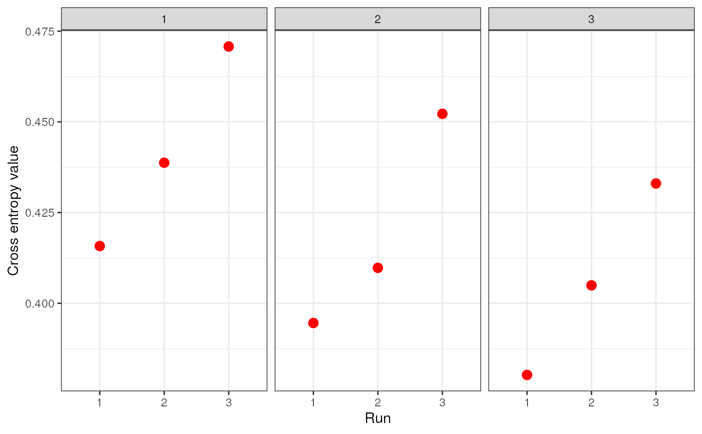
genspecifies the genotype data and can be a dosage matrix, vcfR object, path to vcf file, or an sNMF project (i.e., object of type snmfProject) if you’ve already run SNMF and want to use that for imputationKspecifies a single value or range of K-values for sNMF to be runentropywhether to calculate cross-entropy criteria (defaults to TRUE)repetitionsspecifies the number of repetitions (or runs) to do for each K-value (defaults to 10)projectspecifies whether you want to start a new sNMF project ("new"; default), whether you want to continue an existing SNMF project ("continue") or overwrite existing results ("force")quietproduces a plot of the cross-entropy scores for each K value from sNMF, if set to FALSE. The default is for nothing to be printed (quiet = TRUE). The best K value from the sNMF results is based on minimizing cross-entropy scoressave_outputspecifies whether you would like output files to be saved to file (a string) or not (left NULL; this is the default). If a string is provided, output files will be saved with this argument’s string as a prefix. Files to be saved include SNMF results, the original dosage matrix as .geno and .lfmm files, and an imputed .lfmm file
str_dos <- str_impute(gen = dosage, K = 1:3, entropy = TRUE, repetitions = 3, quiet = FALSE, save_output = FALSE)


Let’s take a look at how the two imputation methods compare by
calculating genetic distances for each and then using the
gen_dist_corr() function which plots the relationship
between two distance metrics (please see the genetic distances vignette
for further information).
str_dist <- as.matrix(ecodist::distance(str_dos, method = "euclidean"))
simple_dist <- as.matrix(ecodist::distance(simple_dos, method = "euclidean"))
gen_dist_corr(dist_x = simple_dist, dist_y = str_dist, metric_name_x = "simple", metric_name_y = "SNMF")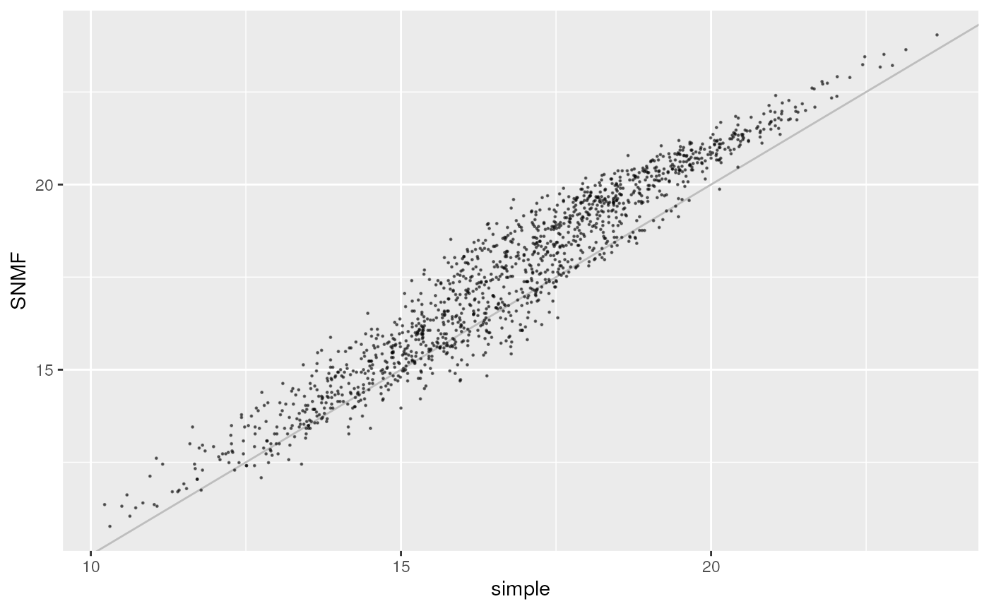
Removing sites that are in linkage disequilibrium using
ld_prune()
For some analyses, we may want to prune out any linked sites from our data to not bias results. This is particularly the case with methods that estimate population structure (e.g., TESS), as population structure can be overinflated as more SNPs appear to independently support the same pattern. For other analyses - such as genotype-environment association methods like RDA and LFMM - SNPs in LD are sometimes removed prior to running such analyses, but we do not recommend this because SNPs most strongly associated with environmental variables may have been pruned out. However, failing to account for linkage may result in overinflated conclusions about environmental associations. A solution to this is to perform LD-pruning after having run GEA methods; one approach to do so is to retain SNPs with the strongest association (i.e., lowest p-value) and removing all others that are in linkage with that particular SNP (see the approach described in Capblancq & Forester 2021 for more information).
To perform LD-pruning, we can use the ld_prune()
function (which largely uses the snpgdsLDpruning() function
within the SNPRelate package). The function works by first removing any
variants that occur below a given minor allele frequency, and then by
pruning any variants that have a given correlation using a sliding
window approach.
The main arguments within this function are as follows:
ld.thresholdspecifies the LD pruning threshold (the default is the correlation coefficient value; thus, the higher theld.thresholdvalue, fewer variants will be pruned)slide.max.nspecifies the maximum number of SNPs in the sliding window (defaults to 100)mafspecifies the minor allele frequency (defaults to 0.05)vcfspecifies the path to the vcf file that you would like to be prunedout_namespecifies the prefix of output file namesout_formatspecifies the file type (options are"vcf"for vcf and gds files [default], or"plink"for ped and map files)save_outputspecifies whether you would like a new directory made containing all output (and intermediate) files; default isTRUE.If set toFALSE, the function will simply return a vcf object.
The way to call this function is as follows:
vcf_ldpruned <- ld_prune(vcf = "test.vcf", out_name = "liz", out_format = "vcf", ld.threshold = 0.9, slide.max.n = 10)
We will not be running this function within the vignette to avoid
generating intermediate files, but the example line above creates a new
directory called liz_LDpruned, and it contains five files: a LOGFILE,
with information on how many sites were pruned and how many remain,
three gds files (pre- and post-pruned SNP GDS files and a GDS SeqArray
file), and the pruned vcf. All of these output files are named such that
the ld.threshold and slide.max.n parameter
settings are contained in file names.
Additional options for data visualization
An alternate way to visualize matrices that can be helpful when you
have many overlapping data points is using the geom_hex()
function in the ggplot2 package. This plotting style bins data points
into hexagons that are colorized based on the number of data points
contained within the hexagon.
Let’s take a look at this style of plot using the comparison between
imputed genetic distances we generated earlier in this vignette. To
makes things easy, let’s re-run the gen_dist_corr()
function and extract the data from the output. This way, it’s already
been processed for us.
if (!require("hexbin", quietly = TRUE)) install.packages("hexbin")
library(hexbin)
# Gather data
plot <- gen_dist_corr(dist_x = simple_dist, dist_y = str_dist, metric_name_x = "simple", metric_name_y = "SNMF")

# Now, build plot
ggplot(plot$data, aes(x = simple, y = SNMF) ) +
  geom_hex() +
  theme_bw() +
  scale_fill_continuous(type = "viridis")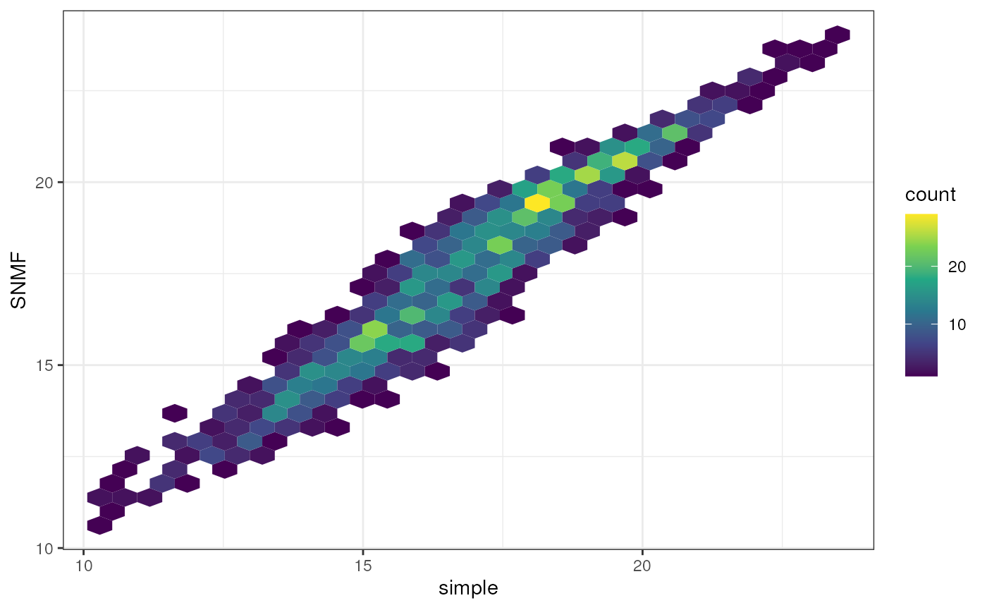
Additional documentation and citations
| Citation/URL | Details | |
|---|---|---|
| Associated code | Zheng et al. 2012; further details here | algatr uses the snpgdsLDpruning() function within the
SNPRelate package for LD-pruning |
Retrieve SNPRelate’s vignette:
vignette("SNPRelate")
#> starting httpd help server ... done